Approximations for Binary Gaussian Process Classification

Approximations for Binary Gaussian Process Classification

Hannes Nickisch [email protected]

Max Planck Institute for Biological Cybernetics Spemannstraße 38

72076 Tübingen, Germany

Carl Edward Rasmussen∗ [email protected]

Department of Engineering University of Cambridge Trumpington Street Cambridge, CB2 1PZ, UK

Editor: Carlos Guestrin

Abstract

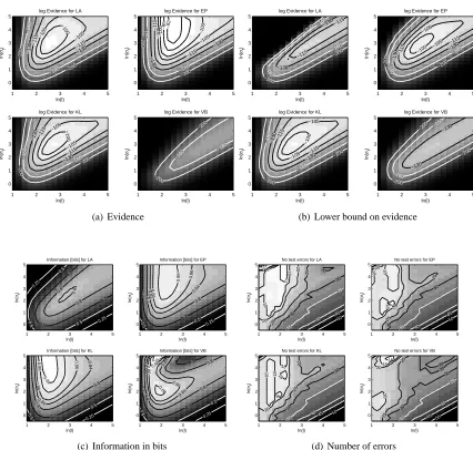
We provide a comprehensive overview of many recent algorithms for approximate inference in Gaussian process models for probabilistic binary classification. The relationships between several approaches are elucidated theoretically, and the properties of the different algorithms are corrobo-rated by experimental results. We examine both 1) the quality of the predictive distributions and 2) the suitability of the different marginal likelihood approximations for model selection (selecting hyperparameters) and compare to a gold standard based on MCMC. Interestingly, some methods produce good predictive distributions although their marginal likelihood approximations are poor. Strong conclusions are drawn about the methods: The Expectation Propagation algorithm is almost always the method of choice unless the computational budget is very tight. We also extend existing methods in various ways, and provide unifying code implementing all approaches.

Keywords: Gaussian process priors, probabilistic classification, Laplaces’s approximation, ex-pectation propagation, variational bounding, mean field methods, marginal likelihood evidence, MCMC

1. Introduction

Gaussian processes (GPs) can conveniently be used to specify prior distributions for Bayesian infer-ence. In the case of regression with Gaussian noise, inference can be done simply in closed form, since the posterior is also a GP. For non-Gaussian likelihoods, such as e.g., in binary classification, exact inference is analytically intractable.

One prolific line of attack is based on approximating the non-Gaussian posterior with a tractable Gaussian distribution. One might think that finding such an approximating GP is a well-defined problem with a largely unique solution. However, we find no less than three different types of solu-tion in the recent literature: Laplace Approximasolu-tion (LA) (Williams and Barber, 1998), Expectasolu-tion Propagation (EP) (Minka, 2001a) and Kullback-Leibler divergence (KL) minimization (Opper and Archambeau, 2008) comprising Variational Bounding (VB) (Gibbs and MacKay, 2000) as a special

case. Another approach is based on a factorial approximation, rather than a Gaussian (Csató et al., 2000).

Practical applications reflect the richness of approximate inference methods: LA has been used for sequence annotation (Altun et al., 2004) and prostate cancer prediction (Chu et al., 2005), EP for affect recognition (Kapoor and Picard, 2005), VB for weld cracking prognosis (Gibbs and MacKay, 2000), Label Regression (LR) serves for object categorization (Kapoor et al., 2007) and MCMC sampling is applied to rheuma diagnosis (Schwaighofer et al., 2002). Brain computer interfaces (Zhong et al., 2008) even rely on several (LA, EP, VB) methods.

In this paper, we compare these different approximations and provide insights into the strengths and weaknesses of each method, extending the work of Kuss and Rasmussen (2005) in several di-rections: We cover many more approximation methods (VB,KL,FV,LR), put all of them in common framework and provide generic implementations dealing with both the logistic and the cumula-tive Gaussian likelihood functions and clarify the aspects of the problem causing difficulties for each method. We derive Newton’s method for KL and VB. We show how to accelerate MCMC simulations. We highlight numerical problems, comment on computational complexity and supply runtime measurements based on experiments under a wide range of conditions, including different likelihood and different covariance functions. We provide deeper insights into the methods behavior by systematically linking them to each other. Finally, we review the tight connections to methods from the literature on Statistical Physics, including the TAP approximation and TAPnaive.

The quantities of central importance are the quality of the probabilistic predictions and the suit-ability of the approximate marginal likelihood for selecting parameters of the covariance function (hyperparameters). The marginal likelihood for any Gaussian approximate posterior can be lower bounded using Jensen’s inequality, but the specific approximation schemes also come with their own marginal likelihood approximations.

We are able to draw clear conclusions. Whereas every method has good performance under some circumstances, only a single method gives consistently good results. We are able to theoreti-cally corroborate our experimental findings; together this provides solid evidence and guidelines for choosing an approximation method in practice.

2. Gaussian Processes for Binary Classification

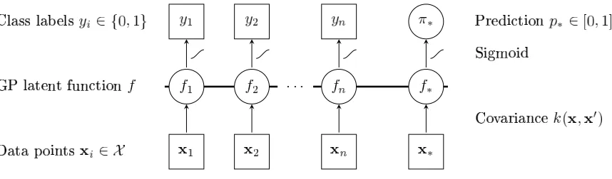
We describe probabilistic binary classification based on Gaussian processes in this section. For a graphical model representation see Figure 1 and for a 1d pictorial description consult Figure 2.

Given data points xi from a domain

X

like to predict the class membership probability for a test point x_∗. This is achieved by using a

latent function f whose value is mapped into the unit interval by means of a sigmoid function

sig :R_→[0,1]such that the class membership probabilityP(y= +1_|x)can be written as sig(f(x)).

The class membership probability must normalize∑yP(y|x) =1, which leads toP(y= +1|x) =1−

P(y=₋1_|x). If the sigmoid function satisfies the point symmetry condition sig(t) =1₋sig(₋t),

the likelihood can be compactly written as

In this paper, two point symmetric sigmoids are considered

sig_logit(t) := 1

1+e−t

sig_probit(t) :=

Z t

−∞

N

The two functions are very similar at the origin (showing locally linear behavior around sig(0) =

1/2 with slope 1/4 for sig_logitand 1/√2πfor sig_probit) but differ in how fast they approach 0/1 when

t goes to infinity. For large negative values of t, we have the asymptotics

sig_logit(t) _≈ exp(₋t) and sig_probit(t) _≈ exp(₋1

2t

2_+0.158t

−1.78), for t0.

Linear decay of ln(sig_logit) corresponds to a weaker penalty for wrongly classified examples than

the quadratic decay of ln(sig_probit).

For notational convenience, the following shorthands are used: The matrix X= [x1, . . . ,xn]of

size n_×d collects the training points, the vector y= [y1, . . . ,yn]> of size n_×1 collects the target

values and latent function values are summarized by f= [f1, . . . ,fn]>with fi=f(xi). Observed data

is written as

D

that is, f_∗contains the latent function values for test points[x_∗,1, . . . ,x_∗,m] =X_∗⊂

X

between latent values f and f_∗ at data points x and x_∗ follow the same notation, namely[K_∗∗]_{i j}=

k(x_∗,i,x∗,j),[K∗]i j=k(xi,x∗,j),[k∗]i=k(xi,x∗) and k∗∗=k(x∗,x∗), where[A]i j denotes the entry

Ai j of the matrix A.

Given the latent function f , the class labels are assumed to be Bernoulli distributed and inde-pendent random variables, which gives rise to a factorial likelihood, factorizing over data points (see Figure 1)

P(y_|f) = P(y_|f) =

n

∏

i=1

P(yi|fi) = n

∏

i=1

sig(yifi). (1)

A GP (Rasmussen and Williams, 2006) is a stochastic process fully specified by a mean function

m(x) =E[f(x)]and a positive definite covariance function k(x,x0) =V[f(x),f(x0)]. This means

that a random variable f(x)is associated to every x∈

X

X

the joint distribution P(f_|X,θ) =

N

matrix K. The mean function and covariance functions may depend on additional hyperparameters

θ. For notational convenience we will assume m(x)_≡0 throughout. Thus, the elements of K are

Ki j=k(xi,xj,θ).

By application of Bayes’ rule, one gets an expression for the posterior distribution over the latent values f

P(f_|y,X,θ) = R P(y|f)P(f|X,θ)

P(y_|f)P(f_|X,θ)df =

N

P(y_|X,θ)

n

∏

i=1

sig(yifi), (2)

where Z=P(y_|X,θ) =R

P(y_|f)P(f_|X,θ)df denotes the marginal likelihood or evidence for the

hy-perparameterθ. The joint prior over training and test latent values f and f_∗given the corresponding

P(f_∗,f_|X_∗,X,θ) =

N

f_∗

0,

K K_∗

K>_∗ K_∗∗

.

When making predictions, we marginalize over the training set latent variables

P(f_∗|X_∗,y,X,θ) =

Z

P(f_∗,f_|X_∗,y,X,θ)df=

Z

P(f_∗|f,X_∗,X,θ)P(f_|y,X,θ)df, (3)

where the joint posterior is factored into the product of the posterior and the conditional prior

P(f_∗|f,X_∗,X,θ) =

N

Finally, the predictive class membership probability p_∗:=P(y_∗=1_|x_∗,y,X,θ)is obtained by

aver-aging out the test set latent variables

P(y_∗|x_∗,y,X,θ) =

Z

P(y_∗|f_∗)P(f_∗|x_∗,y,X,θ)d f_∗ =

Z

sig(y_∗f_∗)P(f_∗|x_∗,y,X,θ)d f_∗. (4)

The integral is analytically tractable for sig_probit(Rasmussen and Williams, 2006, Ch. 3.9) and can

be efficiently approximated for sig_logit(Williams and Barber, 1998, App. A).

Figure 1: Graphical Model for binary Gaussian process classification: Circles represent unknown quantities, squares refer to observed variables. The horizontal thick line means fully

connected latent variables. An observed label yiis conditionally independent of all other

nodes given the corresponding latent variable fi. Labels yi and latent function values

fi are connected through the sigmoid likelihood; all latent function values fi are fully

connected, since they are drawn from the same GP. The labels yiare binary, whereas the

prediction p_∗is a probability and can thus have values from the whole interval[0,1].

2.1 Stationary Covariance Functions

encountered in classification. Stationary covariances of the form k(x,x0,θ) =σ2

fg(|x−x0|/`)with

g :R_→Ra monotonously decreasing function1 andθ=_{σf, `}are widely used. The following

section supplies a geometric intuition of that specific prior in the classification scenario by analyzing

the limiting behavior of the covariance matrix K as a function of the length scale`and the limiting

behavior of the likelihood as a function of the latent function scaleσf. A pictorial illustration of the

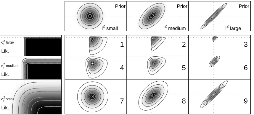
setting is given in Figure 3.

2.1.1 LENGTHSCALE

Two limiting cases of “ignorance with respect to the data” with marginal likelihood Z=2−ncan be

distinguished, where = [1, . . .1]>and I is the identity matrix (see Appendix B.1)

lim

`→0K = σ

2 fI,

lim

`→∞K = σ

2 f

>_.

For very small length scales (`_→0), the prior is simply isotropic as all points are deemed to be

far away from each other and the whole model factorizes. Thus, the (identical) posterior moments can be calculated dimension-wise. (See Figure 3, regimes 1, 4 and 7.)

For very long length scales (`_→∞), the prior becomes degenerate as all datapoints are deemed

to be close to each other and takes the form of a cigar along the hyper-diagonal. (See Figure 3,

regimes 3, 6 and 9.) A 1d example of functions drawn from GP priors with different lengthscales`

is shown in Figure 2 on the left. The lengthscale has to be suited to the data; if chosen too small, we will overfit, if chosen too high underfitting will occur.

2.1.2 LATENTFUNCTIONSCALE

The sigmoid likelihood function sig(yifi)measures the agreement of the signs of the latent function

and the label in a smooth way, that is, values close to one if the signs of yiand fiare the same and|fi|

is large, and values close to zero if the signs are different and_|fi_|is large. The latent function scale

σf of the data can be moved into the likelihood ˜sigσf(t) =sig(σ

2

ft), thusσf models the steepness of

the likelihood and finally the smoothness of the agreement by interpolation between the two limiting cases “ignorant” and “hard cut”

lim

σf→0

sig(t) _≡ 1

2 “ignorant",

lim

σf→∞

sig(t) _≡ step(t):= 0,t<0; 1₂,t=0; 1,0<t “hard cut".

In the case of very small latent scales (σf →0), the likelihood is flat causing the posterior to

equal the prior. The marginal likelihood is again Z=2−n_{. (See Figure 3, regimes 7, 8 and 9.)}

In the case of large latent scales (σf 1), the likelihood approaches the step function. (See

Figure 3, regimes 1, 2 and 3.) A further increase of the latent scale does not change the model

anymore. The model is effectively the same for allσf above a threshold.

0 2 4 6 8 10 −4

−2 0 2 4

a) Prior lengthscales

0 2 4 6 8 10

−4 −2 0 2 4

b) f~Prior

0 2 4 6 8 10

0 0.2 0.4 0.6 0.8 1

c) sig(f), f~Prior

0 2 4 6 8 10 −4

−2 0 2 4

d) f~Posterior, n=7

0 2 4 6 8 10 0

0.2 0.4 0.6 0.8 1

e) sig(f), n=7

0 2 4 6 8 10 −4

−2 0 2 4

f) f~Posterior, n=20

0 2 4 6 8 10 0

0.2 0.4 0.6 0.8 1

g) sig(f), n=20

Figure 2: Pictorial illustration of binary Gaussian process classification in 1d: Plot a) shows 3

sam-ple functions drawn from GPs with different lengthscales`. Then, three pairs of plots

show distributions over functions f :R_→Rand sig(f):R_→[0,1]occurring in GP

clas-sification. b+c) the prior, d+e) a posterior with n=7 observations and f+g) a posterior

with n=20 observations along with the n observations with binary labels. The thick black

line is the mean, the gray background is the_±standard deviation and the thin lines are

sample functions. With more and more data points observed, the uncertainty is gradually shrunk. At the decision boundary the uncertainty is smallest.

2.2 Gaussian Approximations

Unfortunately, the posterior over the latent values (Equation 2) is not Gaussian due to the non-Gaussian likelihood (Equation 1). Therefore, the latent distribution (Equation 3), the predictive distribution (Equation 4) and the marginal likelihood Z cannot be written as analytical expressions. To obtain exact answers, one can resort to sampling algorithms (MCMC). However, if sig is con-cave in the logarithmic domain, the posterior can be shown to be unimodal motivating Gaussian approximations to the posterior. Five different Gaussian approximations corresponding to methods explained later onwards in the paper are depicted in Figure 4.

A quadratic approximation to the log likelihoodφ(fi):=lnP(yi|fi)at ˜fi

φ(fi) ≈ φ(f˜i) +φ0(f˜i)(fi−f˜i) +

1

2φ

00_(f˜_i)(fi−f˜_i)2 ₌

−1₂wifi2+bifi+constfi

motivates the following approximate posteriorQ(f_|y,X,θ)

lnP(f_|y,X,θ) (2)= ₋1

2f

>_K−1_f+

∑

lnP(yi|fi) +constf

quad. approx.

≈ −1₂f>K−1f₋1 2f

>_Wf+b>_f+const

f

m:=(K−1_+W)−1_b

= ₋1

2(f−m)

> _K−1_+W(f

−m) +constf

Prior

l2 small

Prior

l2 medium

Prior

l2 large

Lik. σ_f2

large

Lik. σ_f2 _medium

Lik. σ_f2 _small

1 2 3

4 5 6

7 8 9

Figure 3: Gaussian Process Classification: Prior, Likelihood and exact Posterior: Nine num-bered quadrants show posterior obtained by multiplication of different priors and

like-lihoods. The leftmost column illustrates the likelihood function for three different

steepness parameters σf and the upper row depicts the prior for three different length

scales `. Here, we use σf as a parameter of the likelihood. Alternatively, rows

cor-respond to “degree of Gaussianity” and columns stand for “degree of isotropy“. The

axes show the latent function values f1 = f(x1) and f2= f(x2). A simple toy

exam-ple employing the cumulative Gaussian likelihood and a squared exponential covariance

k(x,x0) =σ2

fexp(− kx−x0k 2

/2`2<sub>) with length scales ln`={0,1,2.5} and latent</sub>

func-tion scales lnσf ={−1.5,0,1.5} is used. Two data points x1 =

√

2, x2=−

√ 2 with

corresponding labels y1=1, y2=−1 form the data set.

where V−1=K−1+W and W denotes the precision of the effective likelihood (see Equation 7). It

turns out that the methods discussed in the following sections correspond to particular choices of m and V.

Let us assume, we have found such a Gaussian approximation to the posterior with mean m and (co)variance V. Consequently, the latent distribution for a test point becomes a tractable one-dimensional Gaussian P(f_∗|x_∗,y,X,θ) =

N

∗) with the following moments (Rasmussen

and Williams, 2006, p. 44 and 56):

µ_∗ = k>_∗K−1m =k>_∗α, α = K−1m, σ2

∗ = k∗∗−k>∗ K−1−K−1VK−1

k_∗ = k_∗∗−k>_∗ K+W−1−1k_∗. (6)

Since Gaussians are closed under multiplication, one can—given the Gaussian priorP(f_|X,θ)

and the Gaussian approximation to the posteriorQ(f_|y,X,θ)—deduce the Gaussian factorQ(y_|f)

sub-best Gaussian posterior, KL=0.118

−5 0 5 10 −10

−5 0 5

LA posterior, KL=0.557

−5 0 5 10 −10

−5 0 5

EP posterior, KL=0.118

−5 0 5 10 −10

−5 0 5

VB posterior, KL=3.546

−5 0 5 10 −10

−5 0 5

KL posterior, KL=0.161

−5 0 5 10 −10

−5 0 5

Figure 4: Five Gaussian Approximations to the Posterior (exact Posterior and mode in gray): Dif-ferent Gaussian approximations to the exact posterior using the regime 2 setting of Figure 3 are shown. The exact posterior is represented in gray by a cross at the mode and a sin-gle equiprobability contour line. From left to right: The best Gaussian approximation (intractable) matches the moments of the true posterior, the Laplace approximation does a Taylor expansion around the mode, the EP approximation iteratively matches marginal moments, the variational method maximizes a lower bound on the marginal likelihood and the KL method minimizes the Kullback-Leibler to the exact posterior. The axes show the latent function values f1= f(x1)and f2= f(x2).

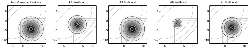
sequently in the paper, are depicted in Figure 5. By “dividing” the approximate Gaussian posterior (see Appendix B.2) by the true Gaussian prior we find the contribution of the effective likelihood

Q(y_|f):

Q(y_|f) ∝

N

N

N

f_|(KW)−1m+m,W−1. (7) We see (also from Equation 5) that W models the precision of the effective likelihood. In general, W

is a full matrix containing n2parameters.2However, all algorithms maintaining a Gaussian posterior

approximation work with a diagonal W to enforce the effective likelihood to factorize over examples (as the true likelihood does, see Figure 1) in order to reduce the number of parameters. We are not aware of work quantifying the error made by this assumption.

2.3 Log Marginal Likelihood

Prior knowledge over the latent function f is encoded in the choice of a covariance function k

con-taining hyperparametersθ. In principle, one can do inference jointly over f andθe.g., by sampling

techniques. Another approach to model selection is maximum likelihood type II also known as

the evidence framework (MacKay, 1992), where the hyperparameters θ are chosen to maximize

the marginal likelihood or evidenceP(y_|X,θ). In other words, one maximizes the agreement

be-tween observed data and the model. Therefore, one has a strong motivation to estimate the marginal likelihood.

Geometrically, the marginal likelihood measures the volume of the prior times the likelihood. High volume implies a strong consensus between our initial belief and our observations. In GP

clas-sification, each data point xi gives rise to a dimension fiin latent space. The likelihood implements

a mechanism, for smoothly restricting the posterior along the axis of fi to the side corresponding

2. Numerical moment matching with K=

7 6

6 7

, y1=y2=1 and sigprobitleads to W=

0.142 −0.017

−0.017 0.142

best Gaussian likelihood

−5 0 5 10 −10

−5 0 5

LA likelihood

−5 0 5 10 −10

−5 0 5

EP likelihood

−5 0 5 10 −10

−5 0 5

VB likelihood

−5 0 5 10 −10

−5 0 5

KL likelihood

−5 0 5 10 −10

−5 0 5

Figure 5: Five Effective Likelihoods (exact Prior/Likelihood in gray): A Gaussian approximation to the posterior induces a Gaussian effective likelihood (Equation 7). Different effective likelihoods are shown; order and setting are the same as described in Figure 4. The axes

show the latent function values f1= f(x1)and f2= f(x2). The effective likelihood

re-places the non-Gaussian likelihood (indicated by three gray lines). A good replacement behaves like the exact likelihood in regions of high prior density (indicated by gray el-lipses). EP and KL yield a good coverage of that region. However LA and VB yield too concentrated replacements.

to the sign of yi . Thus, the latent spaceRnis softly cut down to the orthant given by the values in

y. The log marginal likelihood measures, what fraction of the prior lies in that orthant. Finally, the

value Z=2−ncorresponds to the case, where half of the prior lies on either side along each axis in

latent space. Consequently, successful inference is characterized by Z>2−n.

Some posterior approximations (Sections 3 and 4) provide an approximation to the marginal likelihood, other methods provide a lower bound (Sections 5 and 6). Any Gaussian approximation

Q(f_|θ) =

N

likelihood Z by application of Jensen’s inequality. This bound has been used in the context of sparse approximations (Seeger, 2003).

ln Z=lnP(y_|X,θ) = ln

Z

P(y_|f)P(f_|X,θ)df=ln Z

Q(f_|θ)P(y|f)P(f|X,θ)

Q(f_|θ) df

Jensen

≥ Z

Q(f_|θ)lnP(y|f)P(f|X,θ)

Q(f_|θ) df=: ln ZB. (8)

Some algebra (Appendix B.3) leads to the following expression for ln ZB:

n

∑

i=1

Z

N

Viif+mi df

| {z }

1) data fit

+1

2[n−m

>_K−1_m | {z } 2) data fit

+lnVK−1₋tr VK−1

| {z }

3) regularizer

]. (9)

Model selection means maximization of ln ZB. Term 1) is a sum of one-dimensional Gaussian

of the data-fit term in GP regression (Rasmussen and Williams, 2006, Ch. 5.4.1). Thus, the first

and the second term encourage fitting the data by favouring small variances Viiand large means mi

having the same sign as yi. The third term can be rewritten as−ln|I+KW| −tr (I+KW)−1

and

yields−∑n

i=1ln(1+λi) +1+1λi withλi≥0 being the eigenvalues of KW. Thus, term 3) keeps the

eigenvalues of KW small, thereby favouring a smaller class of functions—this can be seen as an instance of Occam’s razor.

Furthermore, the bound

ln ZB =

Z

Q(f_|θ)lnP(f|y,X,θ)P(y|X)

Q(f_|θ) df =ln Z−KL(Q(f|θ)kP(f|y,X,θ)) (10)

can be decomposed into the exact marginal likelihood minus the Kullback-Leibler (KL) diver-gence between the exact posterior and the approximate posterior. Thus by maximizing the lower

bound ln ZBon ln Z, we effectively minimize the KL-divergence betweenP(f|y,X,θ)andQ(f|θ) =

N

3. Laplace Approximation (LA)

A second order Taylor expansion around the posterior mode m leads to a natural way of constructing

a Gaussian approximation to the log-posteriorΨ(f) =lnP(f_|y,X,θ) (Williams and Barber, 1998;

Rasmussen and Williams, 2006, Ch. 3). The mode m is taken as the mean of the approximate

Gaussian. Linear terms ofΨvanish because the gradient at the mode is zero. The quadratic term of

Ψis given by the negative Hessian W, which - due to the likelihood’s factorial structure - turns out

to be diagonal. The mode m is found by Newton’s method.

3.1 Posterior

P(f_|y,X,θ) _≈

N

N

,

m = argmax

f∈Rn

P(y_|f)P(f_|X,θ),

W = ₋∂

2_lnP(y|f) ∂f∂f>

f=m

=₋

"

∂2_lnP(yi|fi) ∂f_i2

fi=mi

#

ii .

3.2 Log Marginal Likelihood

The unnormalized posterior P(y|f)P(f|X,θ) has its maximum h=exp(Ψ(m)) at its mode m,

where the gradient vanishes. A Taylor expansion ofΨis then given byΨ(f)_≈h₋₂1(f₋m)>(K−1+

W)(f₋m). Consequently, the log marginal likelihood can be approximated by plugging in the

ap-proximation ofΨ(f).

ln Z=lnP(y_|X,θ) = ln

Z

P(y_|f)P(f_|X,θ)df=ln Z

exp(Ψ(f))df

≈ ln h+ln Z

exp

−1

2(f−m)

> _K−1_+W(f−m)

df

= lnP(y_|m)₋1

2m

>_K−1_m+1

4. Expectation Propagation (EP)

EP (Minka, 2001b) is an iterative method to find approximations based on approximate marginal moments, which can be applied to Gaussian processes. See (Rasmussen and Williams, 2006, Ch. 3)

for details. The individual likelihood terms are replaced by site functions ti(fi)being unnormalized

Gaussians

P(yi|fi) ≈ti fi,µi,σ2i,Zi

:= ZiN fi|µi,σ2i

such that the approximate marginal moments of Q(fi):=R

N

(f_|0,K)∏n j=1ZjN

fj|µj,σ2j

df_¬i

agree with the marginals of R

N

(f_|0,K)P(yi_|fi)∏j₆=iZj

N

fj_|µj,σ2j

df_¬i of the approximation

based on the exact likelihood term P(yj|fj). That means, there are 3n quantities µi, σ2i and Zi

to be iteratively optimized. Convergence of EP is not generally guaranteed, but there always exists a fixed-point for the EP updates in GP classification (Minka, 2001a). If the EP iterations converge, the solution obtained is a saddle point of a special energy function (Minka, 2001a). However, an EP update does not necessarily imply a decrease in energy. For our case of log-concave likelihood functions, we always observed convergence, but we are not aware of a formal proof.

4.1 Posterior

Based on these local approximations, the approximate posterior can be written as:

P(f_|y,X,θ) _≈

N

N

,

W = σ−_i 2_ii,

m = VWµ=hI₋K K+W−1−1iKWµ,µ= (µ1, . . . ,µn)>.

4.2 Log Marginal Likelihood

>From the likelihood approximations, one can directly obtain an expression for the approximate log marginal likelihood

ln Z=lnP(y_|X,θ) = ln

Z

P(y_|f)P(f_|X,θ)df

≈ ln

Z n

∏

i=1

t fi,µi,σ2_i,ZiP(f_|X,θ)df

=

n

∑

i=1

ln Zi−

1

2µ

> _K+W−1−1_µ−1

2ln

K+W−1−n

2ln 2π

=

n

∑

i=1

ln_√Zi

2π−

1

2m

> _K−1_+K−1_W−1_K−1_m−1

2ln

K+W−1=: ln ZEP.

The lower bound provided by Jensen’s inequality ZB(Equation 9) is known to be below the

approx-imation ZEP obtained by EP (Opper and Winther, 2005, page 2183). From ZEP≥ZBand Z≥ZBit

is not clear, which value one should use. In principle, ZEPcould be a bad approximation. However,

4.3 Thouless, Anderson & Palmer method (TAP)

Based on ideas rooted in Statistical Physics, one can approach the problem from a slightly different

angle (Opper and Winther, 2000). Individual Gaussian approximations

N

to predictive distributionsP fi|xi,y_\i,X_\i,θ

for data points xithat have been previously removed

from the training set. Based on µ_¬i andσ2_¬i one can derive explicit expressions for(α,W

1 2), our

parameters of interest.

αi _≈

R ∂

∂fiP(yi|fi)

N

2 ¬i)d fi

R

P(yi_|fi)

N

W−1_{ii ≈} σ2_¬i

1

αi[Kα]_i−1

. (11)

In turn, the 2n parameters(µ_¬i,σ2_¬i)can be expressed as a function ofα, K and W

1 2.

σ2

¬i = 1/ h

K+W−1−1

i

ii−

W−1_ii,

µ_¬i = [Kα]_i−σ2_¬iαi. (12)

As a result, a system (Equations 11/12) of nonlinear equations in µ_¬i and σ2_¬i has to be solved

by iteration. Each step involves a matrix inversion of cubic complexity. A faster “naïve” variant updating only n parameters has also been proposed (Opper and Winther, 2000) but it does not lead to the same fixed point. As in the FV algorithm (Section 7), a formal complex transformation leads

to a simplified version by fixingσ2_¬i=Kii, called (TAPnaive) in the sequel.

Finally, for prediction, the predictive posteriorP(f_∗|x_∗,y,X,θ)is approximated by a Gaussian

N

∗)at a test point x∗based on the parameters(α,W

1

2)and according to equation (6).

A fixed-point of the TAP mean-field equations is also a fixed-point of the EP algorithm (Minka, 2001a). This theoretical result was confirmed in our numerical simulations. However, the EP algo-rithm is more practical and typically much faster. For this reason, we are not going to treat the TAP method as an independent algorithm in this paper.

5. KL-Divergence Minimization (KL)

In principle, we simply want to minimize a dissimilarity measure between the approximate posterior

Q(f_|θ) =

N

KL-divergence

KL(P(f_|y,X,θ)_kQ(f_|θ)) =

Z

P(f_|y,X,θ)lnP(f|y,X,θ)

Q(f_|θ) df.

Unfortunately, this expression is intractable. If instead, we measure the reverse KL-divergence, we regain tractability

KL(Q(f_|θ)_kP(f_|y,X,θ)) =

Z

N

N

A similar approach has been followed for regression with Laplace or Cauchy noise (Opper and Archambeau, 2008). Finally, we minimize the following objective (see Appendix B.3) with respect to the variables m and V. Constant terms have been dropped from the expression:

KL(m,V)=c ₋

Z

N

" n

∑

i=1

ln sig(√viiyif+miyi)

#

d f₋1

2ln|V|+ 1

2m

>_K−1_m+1

2tr K

−1_V.

We refer to the first term of KL(m,V)as a(m,V)to keep the expressions short. We calculate first

derivatives and equate them with zero to obtain necessary conditions that have to be fulfilled at a

local optimum(m∗,V∗)

∂KL

∂m =

∂a ∂m−K

−1_m=0

⇒ K−1m= ∂a

∂m=α,

∂KL

∂V =

∂a ∂V+

1

2V

−1₋1

2K

−1_{=0 ⇒ V=}

K−1₋2∂a

∂V

−1

= K−1₋2Λ−1

which definesΛ. If the approximate posterior is parametrized by(m,V), there are in principle in

the order of n2parameters. But if the necessary conditions for a local minimum are fulfilled (i.e., the

derivatives∂KL/∂m and∂KL/∂V vanish), the problem can be re-parametrized in terms of(α,Λ).

Since Λ=∂a/∂V is a diagonal matrix (see Equation 17), the optimum is characterized 2n free

parameters. This fact was already pointed out by Manfred Opper (personal communication) and Matthias Seeger (Seeger, 1999, Ch. 5.21, Eq. 5.3). Thus, a minimization scheme based on Newton iterations on the joint vectorξ:= [α>,Λii]>takes

O

∂KL/∂ξand∂2KL/∂ξ∂ξ> _{are provided in Appendix A.2.}

5.1 Posterior

Based on these local approximations, the approximate posterior can be written as:

P(f_|y,X,θ) _≈

N

N

,

W = ₋2Λ,

m = Kα.

5.2 Log Marginal Likelihood

Since the method inherently maximizes a lower bound on the marginal likelihood, this bound (Equa-tion 9) is used as approxima(Equa-tion to the marginal likelihood.

6. Variational Bounds (VB)

general likelihoods. Individual likelihood bounds

P(yi|fi) ≥ exp aifi2+biyifi+ci

,_∀fi∈R∀i

⇒P(y_|f) _≥ expf>Af+ (by)>f+c> =:Q(y_|f,A,b,c),_∀f_∈R

are defined in terms of coefficients ai,bi and ci, wheredenotes the element-wise product of two

vectors. This lower bound on the likelihood induces a lower bound on the marginal likelihood.

Z=

Z

P(f_|X)P(y_|f)df _≥ Z

P(f_|X)Q(y_|f,A,b,c)df=ZB.

Carrying out the Gaussian integral

ZB =

Z

N

f>Af+ (by)>f+c>

df

leads to (see Appendix B.4)

ln ZB = c> +

1

2(by)

> _K−1

−2A−1(by)₋1

2ln|I−2AK| (13)

which can now be maximized with respect to the coefficients ai,biand ci. In order to get an efficient

algorithm, one has to calculate the first and second derivatives∂ln ZB/∂ς,∂2ln ZB/∂ς∂ς> (as done

in Appendix A.1). Hyperparameters can be optimized using the gradient∂ln ZB/∂θ.

6.1 Logit Bound

Optimizing the logistic likelihood function (Gibbs and MacKay, 2000), we obtain the necessary conditions

Aς := −Λς,

bς :=

1

2 ,

cς,i := ς2iλ(ςi)−

1

2ςi+ln siglogit(ςi)

where we defineλ(ςi) = 2sig_logit(ςi)₋1/(4ςi)andΛς = [λ(ςi)]_ii. This shows, that we only have

to optimize with respect to n parametersς. We apply Newton’s method for this purpose. The bound

is symmetric and tight at f=_±ς.

6.2 Probit Bound

For reasons of completeness, we derive similar expressions (Appendix B.5) for the cumulative

Gaus-sian likelihood sig_probit(fi)with necessary conditions

aς := −

1

2 , (14)

bς,i := ςi+

N

(ςi)

sig_probit(ςi),

cς,i := ςi

2 −bi

ςi+ln sig_probit(ςi)

which again depend only on a single vector of parameters we optimize using Newton’s method. The

6.3 Posterior

Based on these local approximations, the approximate posterior can be written as

P(f_|y,X,θ) _≈

N

N

W = ₋2Aς,

m = V(ybς) = K−1−2Aς

−1

(ybς),

where we have expressed the posterior parameters directly as a function of the coefficients. Finally,

we deal with an approximate posterior Q(f_|θ) =

N

n variational parameters and a mapping ς_7→(mς,Vς). In the KL method, every combination of

values m and W is allowed, in the VB method, mς and Vς cannot be chosen independently, since

the have to be compatible with the bounding requirements. Therefore, the variational posterior is more constrained than the general Gaussian posterior and thus easier to optimize.

6.4 Log Marginal Likelihood

It turns out, that the approximation to the marginal likelihood (Equation 13) is often quite poor and the more general Jensen bound approach (Equation 9) is much tighter. In practice, one would have to evaluate both of them and keep the maximum value.

7. Factorial Variational Method (FV)

Instead of approximating the posteriorP(f_|y,X,θ)by the closest Gaussian distribution, one can use

the closest factorial distributionQ(f|y,X,θ) =∏iQ(fi), also called ensemble learning (Csató et al.,

2000). Another kind of factorial approximationQ(f) =Q(f+)Q(f−)—a posterior factorizing over

classes—is used in multi-class classification (Girolami and Rogers, 2006).

7.1 Posterior

As a result of free-form minimization of the Kullback-Leibler divergence KL(Q(f_|y,X,θ)_kP(f_|y,X,θ))

by equating its functional derivativeδKL/δQ(fi)with the zero function (Appendix B.6), one finds

the best approximation to be of the following form:

Q(fi) ∝

N

P(yi|fi),

µi = mi₋σ2_i K−1m_i= [Kα]_i−σ2_iαi, σ2

i =

K−1−_ii1,

mi =

Z

fiQ(fi)d fi. (15)

it is still possible that the model picks up the most important structure, since the expectations are coupled. Of course, at test time, it is essential that correlations are taken into account again using Equation 6, as it would otherwise be impossible to inject any knowledge into the predictive

dis-tribution. For predictions we use the Gaussian

N

approximation, but it allows to stay inside the Gaussian framework.

Parameters µi and mi are found by the following algorithm. Starting from m=0, iterate the

following until convergence; (1) compute µi, (2) update miby taking a step in the direction towards

mias given by Equation 15. Stepsizes are adapted.

7.2 Log Marginal Likelihood

Surprisingly, one can obtain a lower bound on the marginal likelihood (Csató et al., 2000):

ln Z _≥

n

∑

i=1

ln sig

yimi

σi

−1

2α

>_K−Dg(σ2 1, . . . ,σ2n

>

)α₋1

2ln|K|+

n

∑

i=1

lnσi.

8. Label Regression Method (LR)

Classification has also been treated using label regression or least squares classification (Rifkin and Klautau, 2004). In its simplest form, this method simply ignores the discreteness of the class labels at the cost of not being able to provide proper probabilistic predictions. However, we treat LR

as a heuristic way of choosingα and W, which allows us to think of it as yet another Gaussian

approximation to the posterior allowing for valid predictions of class probabilities.

8.1 Posterior

After inference, according to Equation 6, the moments of the (Gaussian approximation to the) pos-terior GP can be written as µ_∗=k>_∗αandσ2_∗=k_∗∗−k>_∗ K+W−1−1k_∗. Fixing

W−1=σ2_nI and α= K+W−1−1 K+W−1α= K+W−1−1y,

we obtain GP regression from data points xi ∈

X

as a special case. In regression, the posterior moments are given by µ_∗=k>_∗ K+σ2

nI −1

y and

σ2

∗=k∗∗−k>∗ K+σ2nI ₋1

k_∗(Rasmussen and Williams, 2006). The arbitrary scale of the discrete

y can be absorbed by the hyperparameters. There is an additional parameterσn, describing the width

of the effective likelihood. In experiments, we selectedσn_∈[0.5,2]to maximise the log marginal

likelihood.

8.2 Log Marginal Likelihood

There are two ways of obtaining an estimate of the log marginal likelihood. One can simply ignore

the binary nature and use the regression marginal likelihood ln Zregas proxy for ln Z—an approach

we only mention but not use in the experiments

ln Zreg = −

1

2α

> _K+σ2 nI

α₋1

2ln

K+σ2_nI₋n

2ln 2π.

Alternatively, the Jensen bound (8) yields a lower bound ln Z_≥ln ZB—which seems more in line

9. Relations Between the Methods

All considered approximations can be separated into local and global methods. Local methods exploit properties (such as derivatives) of the posterior at a special location only. Global methods

minimize the KL-divergence KL(Q_||P) =R

Q(f)lnQ(f)/P(f)df between the posteriorP(f)and a

tractable family of distributionsQ(f). Often this methodology is also referred to as a variational

algorithm.

assumption relation conditions approx. posteriorQ(f) name

Q(f) =

N

W = ₋∂2_∂ln_f∂P_f(_>y|f)

N

1_+W)−1_{) LA}

Q(f) =∏iqi(fi) _{→ δ}δ_qKL

i(fi)≡0 ∏i

N

2

i)P(yi|fi) FV

&

f_id_q

i(fi)=

f_id_Q(f

i)

N

−1_+W)−1 _EP

%

Q(f) =

N

∂V,m =0

N

1_+W)−1 _KL

&

P(yi_|fi)_≥

N

2

ςi) →

∂KL

∂ς_∗ =0

N

1_+W

ς_∗)−1

VB

P(yi|fi):=

N

N

The only local method considered is the LA approximation matching curvature at the posterior mode. Common tractable distributions for global methods include factorial and Gaussian distri-butions. They have their direct correspondent in the FV method and the KL method. Individual likelihood bounds make the VB method a more constrained and easier-to-optimize version of the KL method. Interestingly, EP can be seen in some sense as a hybrid version of FV and KL, com-bining the advantages of both methods. Within the Expectation Consistence framework (Opper and Winther, 2005), EP can be thought of as an algorithm that implicitly works with two distributions—a

factorial and a Gaussian—having the same marginal momentsf_id. By means of iterative updates,

one keeps these expectations consistent and produces a posterior approximation.

In the divergence measure and message passing framework (Minka, 2005), EP is cast as a mes-sage passing algorithm template: Iterative minimization of local divergences to a tractable family of distributions yields a small global divergence. From that viewpoint, FV and KL are considered

as special cases with divergence measure KL(Q_||P)combined with factorial and Gaussian

distribu-tions.

There is also a link between local and global methods, namely from the KL to the LA method. The necessary conditions for the LA method do hold on average for the KL method (Opper and Archambeau, 2008).

10. Markov Chain Monte Carlo (MCMC)

The only way of getting a handle on the ground truth for the moments Z, m and V is by applying sampling techniques. In the limit of long runs, one is guaranteed to get the right answer. But in practice, these methods can be very slow, compared to analytic approximations discussed previ-ously. MCMC runs are rather supposed to provide a gold standard for the comparison of the other methods.

It turns out to be most challenging to obtain reliable marginal likelihood estimates as it is equiv-alent to solving the free energy problem in physics. We employ Annealed Importance Sampling (AIS) and thermodynamic integration to yield the desired marginal likelihoods. Instead of starting annealing from the prior distribution, we propose to directly start from an approximate posterior in order to speed up the sampling process.

Accurate estimates of the first and second moments can be obtained by sampling directly from the (unnormalized) posterior using Hybrid Monte Carlo methods (Neal, 1993).

10.1 Thermodynamic Integration

The goal is to calculate the marginal likelihood Z=R

P(y_|f)P(f_|X)df. AIS (Neal, 1993, 2001)

works with intermediate quantities Zt :=

R

P(y_|f)τ(t)P(f_|X)df. Here, τ:N_⊃[0,T]_→[0,1]_⊂R

denotes an inverse temperature schedule with the propertiesτ(0) =0,τ(T) =1 andτ(t+1)_≥τ(t)

leading to Z0=RP(f|X)df=1 and ZT=Z.

On the other hand, we have Z=ZT/Z0 =∏Tt=1Zt/Zt−1—an expanded fraction. Each factor

Zt/Zt₋1can be approximated by importance sampling with samples fsfrom the “intermediate

pos-terior”P(f_|y,X,t₋1):=P(y_|f)τ(t−1)P(f_|X)/Zt₋1at time t. Zt

Zt−1

=

R

P(y_|f)τ(t)P(f_|X)df

Zt−1

=

Z _P(_y|_f)τ(t)

P(y_|f)τ(t−1)

P(y_|f)τ(t−1)P(f_|X)

Zt−1

df

=

Z

P(y_|f)∆τ(t)P(f_|y,X,t₋1)df

≈ 1_S

S

∑

s=1

P(y_|fs)∆τ(t), fs∼P(f|y,X,t−1).

This works fine for small temperature changes∆τ(t):=τ(t)₋τ(t₋1). In the limit, we smoothly

interpolate betweenP(y_|f)0P(f_|X)andP(y_|f)1P(f_|X), that is, we start by sampling from the prior and finally approach the posterior. Note that sampling is algorithmically possible even though the distribution is only known up to a constant factor.

10.2 Amelioration Using an Approximation to the Posterior

In practice, the posterior can be quite different from the prior. That means that individual fractions

Zt/Zt−1may be difficult to estimate. One can make these fractions more similar by increasing the

number of steps T or by “starting” from a distribution close to the posterior rather than from the prior. LetQ(f) =

N

N

For the integration we use Zt=RP(y|f)τ(t)Q(y|f)1−τ(t)P(f|X)df where Z0=RQ(y|f)P(f|X)df

can be computed analytically. Again, each factor Zt

by importance sampling from the modified intermediate posterior:

P(f_|y,X,t₋1) = P(y_|f)τ(t−1)Q(y_|f)1−τ(t−1)P(f_|X)/Zt−1

=

P(y_|f)

Q(y_|f)

τ(t−1)

Q(y|f)P(f|X)/Zt₋1,

Zt Zt−1

=

R

P(y_|f)τ(t)Q(y_|f)1−τ(t)P(f_|X)df

Zt−1

=

Z _P(_y|_f)τ(t)_Q(_y|_f)1−τ(t)

P(y_|f)τ(t−1)Q(y_|f)1−τ(t−1)

P(y|f)τ(t−1)Q(y|f)1−τ(t−1)P(f|X)

Zt₋1

df

=

Z _P(_y|_f)

Q(y_|f)

∆τ(t)

P(f|y,X,t−1)df

≈ 1_S

S

∑

s=1

P(y_|fs) Q(y_|fs)

∆τ(t)

, fs∼P(f|y,X,t−1).

The choice ofQ(f)to be a good approximation to the true posterior makes the fractionP(y_|f)/Q(y_|f)

as constant as possible, which in turn reduces the error due to the finite step size in thermodynamical integration.

10.3 Algorithm

If only one sample ftis used per temperatureτ(t), the value of the entire fraction is obtained as

ln Zt

Zt₋1

=∆τ(t) [lnP(y_|ft)−lnQ(y|ft)]

which gives rise to the full estimate

ln Z≈

T

∑

t=1

ln Zt

Zt₋1

=ln ZQ+

T

∑

t=1 ∆τ(t)

lnP(y|ft) +

1

2(ft−m˜)

>_W(f t−m˜)

for a single run r. The finite temperature change bias can be removed by combining results Zrfrom

R different runs by their arithmetic mean 1_R∑rZr(Neal, 2001)

ln Z=ln

Z

P(y_|f)P(f_|X)df_≈ln 1

R R

∑

r=1 Zr

! .

Finally, the only primitive needed to obtain MCMC estimates of Z, m and V is an efficient

sampler for the “intermediate” posterior P(f|y,X,t−1). We use Hybrid Monte Carlo sampling

(Neal, 1993).

10.4 Results

(regimes 4-6), but is sufficiently different from the prior, then the method decreases variance and consequently improves runtimes of AIS. Different approximation methods lead also to differences in the improvement. Namely, the Laplace approximation performs worse than the approximation found by Expectation Propagation because Laplace’s method approximates around the mode which can be far away from the mean.

For our evaluations of the approximations to the marginal likelihood, however we started the algorithm from the prior. Otherwise, one might be worried of biasing the MCMC simulation towards the initial distribution in cases where the chain fails to mix properly.

11. Implementation

Implementations of all methods discussed are provided athttp://www.kyb.mpg.de/~hn/approxXX.

tar.gz. The code is designed as an extension to the Gaussian Processes for Machine Learning

(GPML) (Rasmussen and Williams, 2006) Matlab Code.3 Approximate inference for Gaussian

processes is done by the binaryGP.m function, which takes as arguments the covariance

func-tion, the likelihood function and the approximation method. The existing GPML package provides

approxLA.mfor Laplace’s method andapproxEP.mfor Expectation Propagation. These

implemen-tations are generic to the likelihood function. We providecumGauss.mandlogistic.mthat were

designed to avoid numerical problems. In the extension,approxKL.m,approxVB.m,approxFV.m

andapproxTAP.mare included, among others not discussed here, for example sparse and online

methods outside the scope of the current investigation. The implementations are straight-forward, although special care has been taken to avoid numerical problems e.g., situations where K is close

to singular. More concretely, we use the well-conditioned matrix4 B=W12KW

1

2+I=LL> and

its Cholesky decomposition to calculate V= K−1+W−1or k_∗> K+W−1−1k_∗. The posterior

mean is represented in terms ofαto avoid multiplications with K−1and facilitate predictions.

Especially LA and EP show a high level of robustness along the full spectrum of possible hyper-parameters. KL uses Gauss-Hermite quadrature; we did not notice problems stemming therefrom.

The FV and TAP methods work very reliably, although, we had to add a small (10−6) ridge for FV

to regularize K. As a general statement, we did not observe any numerical problems for a wide range of hyperparameters reaching from reasonable values to very extreme scales.

In addition to the code for the algorithms, we provide also a tarball containing all necessary scripts to reproduce the figures of the paper. We offer two versions: The first version contains only

the code for running the experiments and drawing the figures.5 The second version additionally

includes the results of the experiments.6

12. Experiments

The purpose of the experiments is to illustrate the strengths and weaknesses of the different approxi-mation methods. First of all, the quality of the approxiapproxi-mation itself in terms of posterior moments Z,

3. The package is available athttp://www.gaussianprocess.org/gpml/code. 4. All eigenvaluesλof B satisfy 1≤λ≤1+n

4maxi jKi j, thus B−1and|B|can be safely computed.

5. The code base (∼9Mb) can be obtained fromhttp://www.kyb.mpg.de/~hn/supplement_code.tar.gz. 6. The complete code base (∼400Mb) including all simulation results and scripts to generate figures is stored at

m and V is studied. At a second level, building on the “low-level” features, we compare predictive

performance in terms of the predictive probability p_∗given by (Equations 4 and 6):

p_∗:=P(y_∗=1_|x_∗,y,X,θ) _≈

Z

sig(f_∗)

N

On a third level, we assess higher order properties such as the information score, describing how much information the model managed to extract about the target labels, and the error rate—a binary measure of whether a test input is assigned the right class. Uncertainty predictions provided by the model are not captured by the error rate.

Accurate marginal likelihood estimates Z are a key to hyperparameter learning. In that respect,

Z can be seen as a high-level feature and as the “zeroth” posterior moment at the same time.

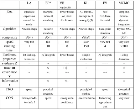
A summary of the whole section is provided in Table 1.

12.1 Data Sets

One main idea of the paper is to study the general behavior of approximate GP classification. Our results for the different approximation methods are not specific to a particular data set but apply to a wide range of application domains. This is reflected by the choice of our reference data sets, widely used in the machine learning literature. Due to limited space, we don’t include the full experiments on all data sets in this paper. However, we have verified that the same qualitative conclusions hold

for all the data sets considered. The full results are available via the web.7

Data set ntrain ntest d Brief description of problem domain

Breast 300 383 9 Breast cancer8

Crabs 100 100 6 Sex of Leptograpsus crabs9

Ionosphere 200 151 34 Classification of radar returns from the ionosphere10

Pima 350 418 8 Diabetes in Pima Indians11

Sonar 108 100 60 Sonar signals bounced by a metal or rock cylinder12

USPS 3 vs. 5 767 773 256 Binary sub-problem of the USPS handwritten digit data set13

12.2 Results

In the following, we report our experimental results covering posterior moments and predictive per-formance. Findings for all 5 methods are provided to make the methods as comparable as possible.

7. See links in Footnotes 5 and 6.

8. Data set athttp://mlearn.ics.uci.edu/databases/breast-cancer-wisconsin/.

9. Data set athttp://www.stats.ox.ac.uk/pub/PRNN/.

10. Data set athttp://mlearn.ics.uci.edu/databases/ionosphere/.

11. Data set athttp://mlearn.ics.uci.edu/databases/pima-indians-diabetes/.

12. Data set at ftp://ftp.ics.uci.edu/pub/machine-learning-databases/undocumented/

connectionist-bench/sonar/.

Training marginals

−200 0 200 −200

0 200

µ for LA

−200 0 200 −200

0 200

µ for EP

−200 0 200 −200

0 200

µ for VB

−200 0 200 −200

0 200

µ for KL

−200 0 200 −200

0 200

µ for FV

0 20 40 0

20 40

σ for LA

0 20 40 0

20 40

σ for EP

0 20 40 0

20 40

σ for VB

0 20 40 0

20 40

σ for KL

0 20 40 0

20 40

σ for FV

0 0.5 1 0

0.5 1

p for LA

0 0.5 1 0

0.5 1

p for EP

0 0.5 1 0

0.5 1

p for VB

0 0.5 1 0

0.5 1

p for KL

0 0.5 1 0

0.5 1

p for FV

Test marginals

−200 0 200 −200

0 200

µ for LA

−200 0 200 −200

0 200

µ for EP

−200 0 200 −200

0 200

µ for VB

−200 0 200 −200

0 200

µ for KL

−200 0 200 −200

0 200

µ for FV

0 20 40 0

20 40

σ for LA

0 20 40 0

20 40

σ for EP

0 20 40 0

20 40

σ for VB

0 20 40 0

20 40

σ for KL

0 20 40 0

20 40

σ for FV

0 0.5 1 0

0.5 1

p for LA

0 0.5 1 0

0.5 1

p for EP

0 0.5 1 0

0.5 1

p for VB

0 0.5 1 0

0.5 1

p for KL

0 0.5 1 0

0.5 1

p for FV

Figure 6: Marginals of USPS 3 vs. 5 for a highly non-Gaussian posterior: Each row consists of five plots showing MCMC ground truth on the x-axis and LA, EP, VB, KL and FV on the y-axis. Based on the logistic likelihood function and the squared exponential

covari-ance function with parameters ln`=2.25 and lnσf =4.25 we plot the marginal means,