Building Blocks for Variational Bayesian Learning of Latent Variable Models

Building Blocks for Variational Bayesian Learning of Latent Variable

Models

Tapani Raiko [email protected]

Harri Valpola [email protected]

Markus Harva [email protected]

Juha Karhunen [email protected]

Adaptive Informatics Research Centre Helsinki University of Technology

P.O.Box 5400, FI-02015 HUT, Espoo, Finland

Editor: Michael I. Jordan

Abstract

We introduce standardised building blocks designed to be used with variational Bayesian learning. The blocks include Gaussian variables, summation, multiplication, nonlinearity, and delay. A large variety of latent variable models can be constructed from these blocks, including nonlinear and variance models, which are lacking from most existing variational systems. The introduced blocks are designed to fit together and to yield efficient update rules. Practical implementation of various models is easy thanks to an associated software package which derives the learning formulas au-tomatically once a specific model structure has been fixed. Variational Bayesian learning provides a cost function which is used both for updating the variables of the model and for optimising the model structure. All the computations can be carried out locally, resulting in linear computational complexity. We present experimental results on several structures, including a new hierarchical nonlinear model for variances and means. The test results demonstrate the good performance and usefulness of the introduced method.

Keywords: latent variable models, variational Bayesian learning, graphical models, building blocks, Bayesian modelling, local computation

1. Introduction

Various generative modelling approaches have provided powerful statistical learning methods for neural networks and graphical models during the last years. Such methods aim at finding an ap-propriate model which explains the internal structure or regularities found in the observations. It is assumed that these regularities are caused by certain latent variables (also called factors, sources, hidden variables, or hidden causes) which have generated the observed data through an unknown mapping (Bishop, 1999). In unsupervised learning, the goal is to identify both the unknown latent variables and generative mapping.

is intractable except in simple toy problems, and hence one must resort to suitable approximations. So-called Laplace approximation (Tierney and Kadane, 1986; Swartz and Evans, 2000) employs a Gaussian approximation around the peak of the posterior distribution. However, this method still suffers from overfitting. In real-world problems, it often does not perform adequately, and has there-fore largely given way for better alternatives. Among them, Markov Chain Monte Carlo (MCMC) techniques (Gelfand and Smith, 1990; Geman and Geman, 1984; Swartz and Evans, 2000) are popu-lar in supervised learning tasks, providing good estimation results. Unfortunately, the computational load is high, which restricts the use of MCMC in large scale unsupervised learning problems where the parameters and variables to be estimated are numerous. For instance, Rowe (2003) has a case study in unsupervised learning from brain imaging data. He used MCMC for a scaled down toy example but resorted to point estimates with real data.

Variational Bayesian learning (Wallace, 1990; Hinton and van Camp, 1993; Neal and Hinton, 1999; Waterhouse et al., 1996; Lappalainen and Miskin, 2000) (for an introduction, see Jordan et al., 1999; MacKay, 2003) has gained increasing attention during the last years. This is because it largely avoids overfitting (Honkela and Valpola, 2004), allows for estimation of the model order and structure, and its computational load is reasonable compared to the MCMC methods. Vari-ational Bayesian learning was first employed in supervised problems (Wallace, 1990; Hinton and van Camp, 1993; MacKay, 1995; Barber and Bishop, 1998), but it has now become popular also in unsupervised modelling. Recently, several authors have successfully applied such techniques to linear factor analysis, independent component analysis (ICA) (Hyv ¨arinen et al., 2001; Roberts and Everson, 2001; Choudrey et al., 2000; Højen-Sørensen et al., 2002), and their various extensions. These include linear independent factor analysis (Attias, 1999), several other extensions of the ba-sic linear ICA model (Attias, 2001; Chan et al., 2001; Miskin and MacKay, 2001; Roberts et al., 2004), mixture models and other graphical models (Attias, 2000; Beal and Ghahramani, 2003; Winn and Bishop, 2005), as well as MLP networks for modelling nonlinear observation mappings (Lap-palainen and Honkela, 2000; Hyv¨arinen et al., 2001) and nonlinear dynamics of the latent variables (source signals) (Ilin et al., 2003; Valpola and Karhunen, 2002; Valpola et al., 2003b). Variational Bayesian learning has also been applied to large discrete models (Murphy, 1999) such as sigmoid belief networks (Jaakkola and Jordan, 1997), nonlinear belief networks (Frey and Hinton, 1999), and hidden Markov models (MacKay, 1997).

The basic building block is a Gaussian variable (node). It uses as its input values both mean and variance. The other building blocks include addition and multiplication nodes, delay, and a Gaussian variable followed by a nonlinearity. Several known model structures can be constructed using these blocks. We also introduce some novel model structures by extending known linear structures using nonlinearities and variance modelling. Examples will be presented later on in this paper.

The key idea behind developing these blocks is that after the connections between the blocks in the chosen model have been fixed (that is, a particular model has been selected and specified), the cost function and the updating rules needed in learning can be computed automatically. The user does not need to understand the underlying mathematics since the derivations are done within the software package. This allows for rapid prototyping. The Bayes Blocks can also be used to bring different methods into a unified framework, by implementing a corresponding structure from blocks and by using results of these methods for initialisation. Different methods can then be compared directly using the cost function and perhaps combined to find even better models. Updates that minimise a global cost function are guaranteed to converge, unlike algorithms such as loopy belief propagation (Pearl, 1988), extended Kalman smoothing (Anderson and Moore, 1979), or expecta-tion propagaexpecta-tion (Minka, 2001).

Winn and Bishop (2005) have introduced a general purpose algorithm called variational mes-sage passing. It resembles our framework in that it uses variational Bayesian learning and factorised approximations. The VIBES framework allows for discrete variables but not nonlinearities or non-stationary variance. The posterior approximation does not need to be fully factorised which leads to a more accurate model. Optimisation proceeds by cycling through each factor and revising the approximate posterior distribution. Messages that contain certain expectations over the posterior approximation are sent through the network.

Beal and Ghahramani (2003); Ghahramani and Beal (2001), and Beal (2003) view variational Bayesian learning as an extension to the EM algorithm. Their algorithms apply to combinations of discrete and linear Gaussian models. In the experiments, the variational Bayesian model structure selection outperformed the Bayesian information criterion (Schwarz, 1978) at relatively small com-putational cost, while being more reliable than annealed importance sampling (Neal, 2001) even with the number of samples so high that the computational cost is hundredfold.

A major difference of our approach compared to the related methods by Winn and Bishop (2005) and by Beal and Ghahramani (2003) is that they concentrate mainly on situations where there is a handy conjugate prior (Gelman et al., 1995) available. This restriction makes computations easier, but on the other hand our blocks can be combined more freely, allowing richer model structures. For instance, the modelling of variance in a way described in Section 5.1, would not be possible using the gamma distribution for the precision parameter in the Gaussian node. The price we have to pay for this advantage is that the minimum of the cost function must be found iteratively, while it can be solved analytically when conjugate distributions are applied. The cost function can always be evaluated analytically in the Bayes Blocks framework as well. Note that the different approaches would fit together.

decision-theoretic nodes. Hence it is in this sense more general than our work. A limitation of the Bayes net toolbox (Murphy, 2001) is that it supports latent continuous nodes only with Gaussian or conditional Gaussian distributions.

Autobayes (Gray et al., 2002) is a system that generates code for efficient implementations of algorithms used in Bayes networks. Currently the algorithm schemas include EM, k-means, and discrete model selection. This system does not yet support continuous hidden variables, nonlinear-ities, variational methods, MCMC, or temporal models. One of the greatest strengths of the code generation approach compared to a software library is the possibility of automatically optimising the code using domain information.

In the independent component analysis (ICA, see textbook by Hyv ¨arinen et al., 2001) commu-nity, traditionally, the observation noise has not been modelled in any way. Even when it is mod-elled, the noise variance is assumed to have a constant value which is estimated from the available observations when required. However, more flexible variance models would be highly desirable in a wide variety of situations. It is well-known that many real-world signals or data sets are nonstation-ary, being roughly stationary on fairly short intervals only. Quite often the amplitude level of a signal varies markedly as a function of time or position, which means that its variance is nonstationary. Examples include financial data sets, speech signals, and natural images.

Recently, Parra, Spence, and Sajda (2001) have demonstrated that several higher-order statis-tical properties of natural images and signals are well explained by a stochastic model in which an otherwise stationary Gaussian process has a nonstationary variance. Variance models are also useful in explaining volatility of financial time series and in detecting outliers in the data. On cer-tain conditions the nonstationarity of variance makes it possible to perform blind source separation (Hyv¨arinen et al., 2001; Pham and Cardoso, 2001).

Several authors have introduced hierarchical models related to those discussed in this paper. These models use subspaces of dependent features instead of single feature components. This kind of models have been proposed at least in context with independent component analysis (Cardoso, 1998; Hyv¨arinen and Hoyer, 2000b,a; Park and Lee, 2004), and topographic or self-organising maps (Kohonen et al., 1997; Ghahramani and Hinton, 1998). A problem with these methods is that it is difficult to learn the structure of the model or to compare different model structures.

The remainder of this paper is organised as follows. In the following section, we briefly present basic concepts of variational Bayesian learning. In Section 3, we introduce the building blocks (nodes), and in Section 4 we discuss variational Bayesian computations with them. In the next section, we show examples of different types of models which can be constructed using the building blocks. Section 6 deals with learning and potential problems related with it, and in Section 7 we present experimental results on several structures given in Section 5. This is followed by a short discussion as well as conclusions in the last section of the paper.

2. Variational Bayesian Learning

In Bayesian data analysis and estimation methods (Gelman et al., 1995),all the uncertain quantities are modelled in terms of their joint probability density function (pdf). The key principle is to con-struct the joint posterior pdf for all the unknown quantities in a model, given the data sample. This posterior density contains all the relevant information on the unknown variables and parameters.

θgiven the data X is obtained from Bayes rule1

p(θ|X,

H

) = p(X |θ,

H

)p(θ|

H

)

p(X|

H

) . (1)

Here p(X|θ,

H

)is the likelihood of the parametersθgiven the data X , p(θ|

H

)is the prior pdf of these parameters, and

p(X|

H

) =

Z

θp(X|θ,

H

)p(θ|

H

)dθ

is a normalising term which is called the evidence. The evidence can be directly understood as the marginal probability of the observed data X assuming the chosen model

H

. By evaluating the evidences p(X|

H

i)for different models

H

i, one can therefore choose the model which describes the observed data with the highest probability (See Valpola and Karhunen, 2002; Bishop, 1995; MacKay, 2003, for a more complete discussion).

Variational Bayesian learning (Wallace, 1990; Hinton and van Camp, 1993; Neal and Hinton, 1999; Waterhouse et al., 1996; Barber and Bishop, 1998; Lappalainen and Miskin, 2000) is a fairly recently introduced approximate fully Bayesian method, which has become popular. Its key idea is to approximate the exact posterior distribution p(θ|X,

H

) by another distribution q(θ) that is computationally easier to handle. The approximating distribution is usually chosen to be a product of several independent distributions, one for each parameter or a set of similar parameters.

Variational Bayesian learning employs the Kullback-Leibler (KL) information (divergence) be-tween two probability distributions q(v)and p(v). The KL information is defined by the cost func-tion

J

KL(qkp) = Z

v

q(v)lnq(v)

p(v)dv (2)

which measures the difference in the probability mass between the densities q(v) and p(v). Its minimum value 0 is achieved when the densities q(v)and p(v)are the same.

The KL information is used to minimise the misfit between the actual posterior pdf p(θ|X,

H

)

and its parametric approximation q(θ). However, the exact KL information

J

KL(q(θ)kp(θ|X,

H

)) between these two densities does not yet yield a practical cost function, because the normalising term p(X|

H

)needed in computing p(θ|X,

H

)cannot usually be evaluated.

Therefore, the cost function used in variational Bayesian learning is defined (Hinton and van Camp, 1993; MacKay, 1995)

C

KL=

J

KL(q(θ)kp(θ|X,

H

))−ln p(X|

H

). (3)

After slight manipulation, this yields

C

KL= Z

θq(θ)ln

q(θ)

p(X,θ|

H

)dθ (4)

which does not require p(X|

H

)any more. The cost function

C

KL=

C

q+

C

pconsists of two parts, the negative entropy

C

qand the expected energy

C

p:

C

q=hln q(θ)i=

Z

θq(θ)ln q(θ)dθ, (5)

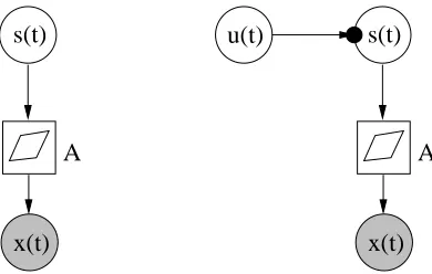
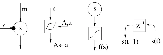
Figure 1: The dash-lined nodes and connections can be ignored while updating the shadowed node. Left: In general, the whole Markov blanket needs to be considered. Right: A completely factorial posterior approximation with no multiple computational paths leads to a decou-pled problem. The nodes can be updated locally.

C

p=

−ln p(X,θ|

H

)= − Z

θq(θ)ln p(X,θ|

H

)dθ (6) where the shorthand notationh·idenotes expectation with respect to the approximate pdf q(θ).

In addition, the cost function

C

KLprovides a bound for the evidence p(X|

H

). Since

J

KL(qkp) is always nonnegative, it follows directly from (3) that

C

KL≥ −ln p(X|

H

).

This shows that the negative of the cost function bounds the log-evidence from below.

It is worth noting that variational Bayesian ensemble learning can be derived from information-theoretic minimum description length coding as well (Hinton and van Camp, 1993). Further con-siderations on such arguments, helping to understand several common problems and certain aspects of learning, have been presented in a recent paper (Honkela and Valpola, 2004).

The dependency structure between the parameters in our method is the same as in Bayesian networks (Pearl, 1988; Bishop, 2006). Variables are seen as nodes of a graph. Each variable is conditioned by its parents. The difficult part in the cost function is the expectationln p(X,θ|

H

)

which is computed over the approximation q(θ)of the posterior pdf. The logarithm splits the prod-uct of simple terms into a sum. If each of the simple terms can be computed in constant time, the overall computational complexity is linear.

In general, the computation time is constant if the parents are independent in the posterior pdf approximation q(θ). This condition is satisfied if the joint distribution of the parents in q(θ)

decouples into the product of the approximate distributions of the parents. That is, each term in q(θ)

−1

z

v

m

s

As+a

_f(s)

s(t−1)

s

A,a

s

s(t)

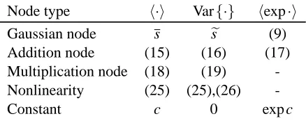
Figure 2: First subfigure from the left: The circle represents a Gaussian node corresponding to the latent variable s conditioned by mean m and variance exp(−v). Second subfigure: Addition and multiplication nodes are used to form an affine mapping from s to As+a. Third subfigure: A nonlinearity f is applied immediately after a Gaussian variable. The rightmost subfigure: Delay operator delays a time-dependent signal by one time unit.

variances measure the reliability of these estimates. However, occasionally the diagonal Gaussian approximation can be too crude. This problem has been considered in context with independent component analysis in Ilin and Valpola (2003), giving means to remedy the situation.

Taking into account posterior dependencies makes the posterior pdf approximation q(θ) more accurate, but also usually increases the computational load significantly. We have earlier consid-ered networks with multiple computational paths in several papers, for example (Lappalainen and Honkela, 2000; Valpola et al., 2002; Valpola and Karhunen, 2002; Valpola et al., 2003b). The com-putational load of variational Bayesian learning then becomes roughly quadratically proportional to the number of unknown variables in the MLP network model used in Lappalainen and Honkela (2000), Valpola et al. (2003b), and Honkela and Valpola (2005).

The building blocks (nodes) introduced in this paper together with associated structural con-straints provide effective means for combating the drawbacks mentioned above. Using them, up-dating at each node takes place locally with no multiple paths. As a result, the computational load scales linearly with the number of estimated quantities. The cost function and the learning formulas for the unknown quantities to be estimated can be evaluated automatically once a specific model has been selected, that is, after the connections between the blocks used in the model have been fixed. This is a very important advantage of the proposed block approach.

3. Node Types

In this section, we present different types of nodes that can be easily combined together. Variational Bayesian inference algorithm for the nodes is then discussed in Section 4.

In general, the building blocks can be divided into variable nodes, computation nodes, and constants. Each variable node corresponds to a random variable, and it can be either observed or hidden. In this paper we present only one type of variable node, the Gaussian node, but others can be used in the same framework. The computation nodes are the addition node, the multiplication node, a nonlinearity, and the delay node.

and its output is the value of the variable. For computation nodes, the output is a fixed function of the inputs. The symbols used for various nodes are shown in Figure 2. Addition and multiplication nodes are not included, since they are typically combined to represent the effect of a linear transfor-mation, which has a symbol of its own. An output signal of a node can be used as input by zero or more nodes that are called the children of that node. Constants are the only nodes that do not have inputs. The output is a fixed value determined at creation of the node.

Nodes are often structured in vectors or matrices. Assume for example that we have a data matrix X= [x(1),x(2), . . . ,x(T)], where t=1,2, . . .T is called the time index of an n-dimensional observation vector. Note that t does not have to correspond to time in the real world, it is just the index of the data case. In the implementation, the nodes are either vectors so that the values indexed by t (observations and latent variables) or scalars so that the values are constants w.r.t. t (parameters). The data X would be represented with n vector nodes. A weight matrix A has to be represented with scalar nodes only. A scalar node can be a parent of a vector node, but not a child of a vector node in this sense. In figures and formulae, we use vectors and matrices more freely.

3.1 Gaussian Node

The Gaussian node is a variable node and the basic element in building hierarchical models. Figure 2 (leftmost subfigure) shows the schematic diagram of the Gaussian node. Its output is the value of a Gaussian random variable s, which is conditioned by the inputs m and v. Denote generally by

N

(x; mx,σ2x)the probability density function of a Gaussian random variable x having the mean mx and varianceσ2_x. Then the conditional probability function (cpf) of the variable s is p(s|m,v) =

N

(s; m,exp(−v)). As a generative model, the Gaussian node takes its mean input m and adds to it Gaussian noise (or innovation) with variance exp(−v).

Variables can be latent or observed. Observing a variable means fixing its output s to the value in the data. Section 4 is devoted to inferring the distribution over the latent variables given the observed variables. Inferring the distribution over variables that are independent of t is also called learning.

3.2 Computation Nodes

The addition and multiplication nodes are used for summing and multiplying variables. These stan-dard mathematical operations are typically used to construct linear mappings between the variables. This task is automated in the software, but in general, the nodes can be connected in other ways, too. An addition node that has n inputs denoted by s1,s2, . . . ,sn, gives the sum of its inputs as the output∑n_i=1si. Similarly, the output of a multiplication node is the product of its inputs∏ni=1si.

A nonlinear computation node can be used for constructing nonlinear mappings between the variable nodes. The nonlinearity

f(s) =exp(−s2) (7)

is chosen because the required expectations can be solved analytically for it. Another implemented nonlinearity for which the computations can be carried out analytically is the cut function g(s) =

3.3 Delay Node

The delay operation can be used to model dynamics. The node operates on time-dependent signals. It transforms the inputs s(1),s(2), . . . ,s(T) into outputs s0,s(1),s(2), . . . ,s(T −1) where s0 is a scalar parameter that provides a starting distribution for the dynamical process. The symbol z−1 in the rightmost subfigure of Fig. 2 illustrating the delay node is the standard notation for the unit delay in signal processing and temporal neural networks (Haykin, 1998). Models containing the delay node are called dynamic, and the other models are called static.

4. Variational Bayesian Inference in Bayes Blocks

In this section we give equations needed for computation with the nodes introduced in Section 3. Generally speaking, each node propagates to the forward direction a distribution of its output given its inputs. In the backward direction, the dependency of the cost function (4) of the children on the output of their parent is propagated. These two potentials are combined to form the posterior distribution of each variable. There is a direct analogy to Bayes rule (1): the prior (forward) and the likelihood (backward) are combined to form the posterior distribution. We will show later on that the potentials in the two directions are fully determined by a few values, which consist of certain expectations over the distribution in the forward direction, and of gradients of the cost function w.r.t. the same expectations in the backward direction.

In the following, we discuss in more detail the properties of each node. Note that the delay node does not actually process the signals, it just rewires them. Therefore no formulas are needed for its associated the expectations and gradients.

4.1 Gaussian Node

Recall the Gaussian node in Section 3.1. The variance is parameterised using the exponential func-tion as exp(−v). This is because then the meanhviand expected exponentialhexp viof the input v suffice for evaluating the cost function, as will be shown shortly. Consequently the cost function can be minimised using the gradients with respect to these expectations. The gradients are computed backwards from the children nodes, but otherwise our learning method differs clearly from standard back-propagation (e.g., Haykin, 1998).

Another important reason for using the parameterisation exp(−v) for the prior variance of a Gaussian random variable s is that the posterior distribution of s then becomes approximately Gaus-sian, provided that the prior mean m of s is GausGaus-sian, too (see for example Section 7.1 or Lap-palainen and Miskin, 2000). The conjugate prior distribution of the inverse of the prior variance of a Gaussian random variable is the gamma distribution (Gelman et al., 1995).

p(x|µ,γ) =

N

x|µ,γ−1, p(γ|a,b) =Gamma(γ|a,b) = b

a

Γ(a)γ

a−1_exp(−bγ).

it should be noted that both the gamma and exp(−v) distributions are used as prior pdfs mainly because they make the estimation of the posterior pdf mathematically tractable (Lappalainen and Miskin, 2000); one cannot claim that either of these choices would be correct.

4.1.1 COSTFUNCTION

Recall now that we are approximating the joint posterior pdf of the random variables s, m, and v in a maximally factorial manner. It then decouples into the product of the individual distributions: q(s,m,v)= q(s)q(m)q(v). Hence s, m, and v are assumed to be statistically independent a posteriori. The posterior approximation q(s) of the Gaussian variable s is defined to be Gaussian with mean s and variancees: q(s) =

N

(s; s,es). Using these, the part

C

pof the Kullback-Leibler cost function arising from the data, defined in Eq. (6), can be computed in closed form. For the Gaussian node of Figure 2, the cost becomes

C

s,p=− hln p(s|m,v)i

=1

2

n

hexp vih(s− hmi)2+Var{m}+es

i

− hvi+ln 2π

o

(8)

The derivation is presented in Appendix B of Valpola and Karhunen (2002) using slightly different notation. For the observed variables, this is the only term arising from them to the cost function

C

KL.

However, latent variables contribute to the cost function

C

KLalso with the part

C

qdefined in Eq. (5), resulting from the expectationhln q(s)i. This term is

C

s,q=

Z

s

q(s)ln q(s)ds=−1

2[ln(2πse) +1]

which is the negative entropy of Gaussian variable with variance es. The parameters defining the approximation q(s)of the posterior distribution of s, namely its mean s and variance es, are to be optimised during learning.

The output of a latent Gaussian node trivially provides the mean and the variance: hsi=s and Var{s}=es. The expected exponential can be easily shown to be (Lappalainen and Miskin, 2000; Valpola and Karhunen, 2002)

hexp si=exp(s+_es/2). (9)

The outputs of the nodes corresponding to the observations are known scalar values instead of distributions. Therefore for these nodes hsi=s, Var{s}=0, andhexp si=exp s. An important conclusion of the considerations presented this far is that the cost function of a Gaussian node can be computed analytically in a closed form. This requires that the posterior approximation is Gaussian and that the meanhmiand the variance Var{m}of the mean input m as well as the mean hviand the expected exponentialhexp viof the variance input v can be computed. To summarise, we have shown that Gaussian nodes can be connected together and their costs can be evaluated analytically.

from Eq. (8), taking the form

∂

C

s,p

∂hmi =hexp vi(hmi −s), (10) ∂

C

s,p

∂Var{m}=

hexp vi

2 , (11)

∂

C

s,p

∂hvi =−

1

2, (12)

∂

C

s,p ∂hexp vi =

(s− hmi)2_+Var{m}+es

2 . (13)

4.1.2 UPDATING THEPOSTERIORDISTRIBUTION

The posterior distribution q(s)of a latent Gaussian node can be updated as follows.

1. The distribution q(s)affects the terms of the cost function

C

sarising from the variable s itself, namely

C

s,p and

C

s,q, as well as the

C

p terms of the children of s, denoted by

C

ch(s),p. The gradients of the cost

C

ch(s),p with respect tohsi, Var{s}, andhexp siare computed according to Equations (10–13).

2. The terms in

C

pwhich depend on s andes can be shown (see Appendix B.2) to be of the form 2

C

p=

C

s,p+

C

ch(s),p=Ms+V[(s−scurrent)2+es] +Ehexp si, (14) where

M=∂

C

p

∂s , V =

∂

C

p

∂se , and E=

∂

C

p ∂hexp si.

3. The minimum of

C

s=

C

s,p+

C

s,q+

C

ch(s),pis solved. This can be done analytically if E =0, corresponding to the case of so-called free-form solution (see Lappalainen and Miskin, 2000, for details):

sopt=scurrent− M

2V , esopt= 1 2V.

Otherwise the minimum is obtained iteratively. Iterative minimisation can be carried out efficiently using Newton’s method for the posterior mean s and a fixed-point iteration for the posterior variances. The minimisation procedure is discussed in more detail in Appendix A._e

4.2 Addition and Multiplication Nodes

Consider first the addition node. The mean, variance and expected exponential of the output of the addition node can be evaluated in a straightforward way. Assuming that the inputs siare statistically

independent, these expectations are respectively given by

*

n

∑

i=1 si

+ =

n

∑

i=1

hsii, (15)

Var

(

n

∑

i=1 si

) =

n

∑

i=1

Var{si}, (16)

*

exp n

∑

i=1 si

!+ =

n

∏

i=1

hexp sii. (17)

The proof has been given in Appendix B.1.

Consider then the multiplication node. Assuming independence between the inputs si, the mean and the variance of the output take the form (see Appendix B.1)

*

n

∏

i=1 si

+ =

n

∏

i=1

hsii, (18)

Var

(

n

∏

i=1 si

) =

n

∏

i=1

h

hsii2+Var{si}

i

− n

∏

i=1

hsii2. (19) For the multiplication node the expected exponential cannot be evaluated without knowing the exact distribution of the inputs.

The formulas (15)–(19) are given for n inputs because of generality, but in practice we have carried out the needed calculations pairwise. When using the general formula (19), the variance might otherwise occasionally take a small negative value due to minor imprecisions appearing in the computations. This problem does not arise in pairwise computations. Now, the propagation in the forward direction is covered.

The form of the cost function propagating from children to parents is assumed to be of the form (14). This is true even in the case, where there are addition and multiplication nodes in between (see Appendix B.2 for proof). Therefore only the gradients of the cost function with respect to the different expectations need to be propagated backwards to identify the whole cost function w.r.t. the parent. The required formulas are obtained in a straightforward manner from Eqs. (15)–(19). The gradients for the addition node are:

∂C ∂hs1i

= ∂C

∂hs1+s2i

, (20)

∂C ∂Var{s1}=

∂C

∂Var{s1+s2}, (21)

∂C

∂hexp s1i=hexp s2i

∂C

∂hexp(s1+s2)i. (22)

For the multiplication node, they become ∂C

∂hs1i =hs2i ∂C

∂hs1s2i+2Var{s2} ∂C

∂Var{s1s2}hs1i, (23) ∂C

∂Var{s1}

=hs2i2+Var{s2} ∂C ∂Var{s1s2}

As a conclusion, addition and multiplication nodes can be added between the Gaussian nodes whose costs still retain the form (14). Proofs can be found in Appendices B.1 and B.2.

4.3 Nonlinearity Node

A serious problem arising here is that for most nonlinear functions it is impossible to compute the required expectations analytically. Here we describe a particular nonlinearity in detail and discuss the options for extending to other nonlinearities, for which the implementation is underway.

Ghahramani and Roweis have shown (1999) that for the nonlinear function f(s) =exp(−s2_)in Eq. (7), the mean and variance have analytical expressions, to be presented shortly, provided that it has Gaussian input. In our graphical network structures this condition is fulfilled if we require that the nonlinearity must be inserted immediately after a Gaussian node. The same type of exponential function (7) is frequently used in standard radial-basis function networks (Bishop, 1995; Haykin, 1998; Ghahramani and Roweis, 1999), but in a different manner. There the exponential function depends on the Euclidean distance from a centre point, while in our case it depends on the input variable s directly.

The first and second moments of the function (7) with respect to the distribution q(s) are (Ghahramani and Roweis, 1999)

hf(s)i=exp

− s 2 2se+1

(2se+1)−12, (25)

[f(s)]2=exp

− 2s 2 4se+1

(4se+1)−12. ₍₂₆₎

The formula (25) provides directly the mean hf(s)i, and the variance is obtained from (25) and (26) by applying the familiar formula Var{f(s)}=[f(s)]2_{− hf(s)i}2

. The expected exponential hexp f(s)icannot be evaluated analytically, which limits somewhat the use of the nonlinear node.

The updating of the nonlinear node following directly a Gaussian node takes place similarly as the updating of a plain Gaussian node. The gradients of

C

p with respect tohf(s)iand Var{f(s)} are evaluated assuming that they arise from a quadratic term. This assumption holds since the nonlinearity can only propagate to the mean of Gaussian nodes. The update formulas are given in Appendix C.

Another possibility is to use as the nonlinearity the error function f(s)=Rs

−∞exp(−r2)dr,

be-cause its mean can be evaluated analytically and variance approximated from above (Frey and Hin-ton, 1999). Increasing the variance increases the value of the cost function, too, and hence it suffices to minimise the upper bound of the cost function for finding a good solution. Frey and Hinton (1999) apply the error function in MLP (multilayer perceptron) networks (Bishop, 1995; Haykin, 1998) but in a manner different from ours.

Finally, Murphy (1999) has applied the hyperbolic tangent function f(s) = tanh(s), approxi-mating it iteratively with a Gaussian. Honkela and Valpola (2005) approximate the same sigmoidal function with a Gauss-Hermite quadrature. This alternative could be considered here, too. A prob-lem with it is, however, that the cost function (mean and variance) cannot be computed analytically.

4.4 Other Possible Nodes

Node type h·i Var{·} hexp·i

Gaussian node s es (9)

Addition node (15) (16) (17) Multiplication node (18) (19) -Nonlinearity (25) (25),(26)

-Constant c 0 exp c

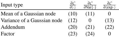
Table 1: The forward messages or expectations that are provided by the output of different types of nodes. The numbers in parentheses refer to defining equations. The multiplication and nonlinearity cannot provide the expected exponential.

the rectified Gaussian node. MoG can be used to model any sufficiently well behaving distribution (Bishop, 1995). In the independent factor analysis (IFA) method introduced in Attias (1999), a MoG distribution was used for the sources, resulting in a probabilistic version of independent component analysis (ICA) (Hyv¨arinen et al., 2001).

The second new node type, the rectified Gaussian variable, was introduced in Miskin and MacKay (2001). By omitting negative values and retaining only positive ones of a variable which is originally Gaussian distributed, this block allows modelling of variables having positive values only. Such variables are commonplace for example in digital image processing, where the picture elements (pixels) have always non-negative values. The cost functions and update rules of the MoG and rectified Gaussian node have been derived by Harva (2004). We postpone a more detailed discussion of these nodes to forthcoming papers to keep the length of this paper reasonable.

In the early conference paper (Valpola et al., 2001) where we introduced the blocks for the first time, two more blocks were proposed for handling discrete models and variables. One of them is a switch, which picks up its k-th continuous valued input signal as its output signal. The other one is a discrete variable k, which has a soft-max prior derived from the continuous valued input signals ci of the node. However, we have omitted these two nodes from the present paper, because their performance has not turned out to be adequate. The reason might be that assuming posterior independence of the auxiliary Gaussian variables is too rough and that the cost function in the soft-max case could not be computed exactly. For instance, building a mixture-of-Gaussians from discrete and Gaussian variables with switches is possible, but the construction loses out to a specialised MoG node that makes fewer assumptions. Raiko (2005) uses the soft-max node without switches.

Action and utility nodes (Pearl, 1988; Murphy, 2001) would extend the library into decision theory and control. In addition to the messages about the variational Bayesian cost function, the network would propagate messages about utility. Raiko and Tornio (2005) describe such a system in a slightly different framework.

5. Combining the Nodes

Input type _∂∂_h·iC _∂Var∂C_{{·} ∂hexp}∂C_·i Mean of a Gaussian node (10) (11) 0 Variance of a Gaussian node (12) 0 (13)

Addendum (20) (21) (22)

Factor (23) (24) 0

Table 2: The backward messages or the gradients of the cost function w.r.t. certain expectations. The numbers in parentheses refer to defining equations. The gradients of the Gaussian node are derived from Eq. (8). The Gaussian node requires the corresponding expecta-tions from its inputs, that is,hmi, Var{m}, hvi, andhexp vi. Addition and multiplication nodes require the same type of input expectations that they are required to provide as output. Communication of a nonlinearity with its Gaussian parent node is described in Appendix C.

When connecting the nodes, the following restrictions must be taken into account:

1. In general, the network has to be a directed acyclic graph (DAG). The delay nodes are an exception because the past values of any node can be the parents of any other nodes. This violation is not a real one in the sense that if the structure were unfolded in time, the resulting network would again be a DAG.

2. The nonlinearity must always be placed immediately after a Gaussian node. This is because the output expectations, Equations (25) and (26), can be computed only for Gaussian inputs. The nonlinearity also breaks the general form of the likelihood (14). This is handled by using special update rules for the Gaussian followed by a nonlinearity (Appendix C).

3. The outputs of multiplication and nonlinear nodes cannot be used as variance inputs for the Gaussian node. This is because the expected exponential cannot be evaluated for them. These restrictions are evident from Tables 1 and 2.

4. There should be only one computational path from a latent variable to a variable. A compu-tational path is a path that consists of computation nodes only. Otherwise, the independency assumptions used in Equations (8) and (16)–(19) are violated and variational Bayesian learn-ing becomes more complicated (recall Figure 1).

Figure 3 shows examples of model structures that break each of the restrictions in turn. The software package includes a function that checks whether a given model structure is correct or not. Note that the network may contain loops, that is, the underlying undirected network can be cyclic. Note also that the second, third, and fourth restrictions can be circumvented by inserting mediating Gaussian nodes. A mediating Gaussian node that is used as the variance input of another variable, is called the variance source and it is discussed in the following.

5.1 Nonstationary Variance

4.

1.

2.

3.

Figure 3: Examples of illegal model structures violating each of the restriction described in the text in turn.

m

v

m

v

s(t)

w

u(t)

s(t)

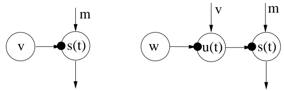
Figure 4: Left: The Gaussian variable s(t)has a a constant variance exp(−v)and mean m. Right: A variance source is added for providing a non-constant variance input u(t)to the output (source) signal s(t). The variance source u(t) has a prior mean v and prior variance exp(−w).

model it. For modelling the variance, too, we use the variance source (Valpola et al., 2004) depicted schematically in Figure 4. Variance source is a regular Gaussian node whose output u(t)is used as the input variance of another Gaussian node. Variance source can convert prediction of the mean into prediction of the variance, allowing to build hierarchical or dynamical models for the variance.

Var{u(t)}=0 Var{u(t)}=1 Var{u(t)}=2

Figure 5: The distribution of s(t)is plotted when s(t)∼

N

(0,exp[−u(t)])and u(t)∼

N

(0,·). Note that when Var{u(t)}=0, the distribution of s(t)is Gaussian. This corresponds to the right subfigure of Fig. 4 when m=v=0 and exp(−w) =0,1,2.

5.2 Linear Independent Factor Analysis

In many instances there exist several nodes which have quite similar role in the chosen structure. Assuming that ithsuch node corresponds to a scalar variable yi, it is convenient to use the vector y = (y1,y2, . . . ,yn)T to jointly denote all the corresponding scalar variables y1,y2, . . . ,yn. This notation is used in Figures 6 and 7 later on. Hence we represent the scalar source nodes corresponding to the variables si(t)using the source vector s(t), and the scalar nodes corresponding to the observations xi(t)using the observation vector x(t).

The addition and multiplication nodes can be used for building an affine transformation

x(t) =As(t) +a+nx(t) (27)

from the Gaussian source nodes s(t)to the Gaussian observation nodes x(t). The vector a denotes the bias and vector nx(t)denotes the zero-mean Gaussian noise in the Gaussian node x(t). This model corresponds to standard linear factor analysis (FA) assuming that the sources si(t)are mutu-ally uncorrelated; see for example, Hyv¨arinen et al. (2001).

If instead of Gaussianity it is assumed that each source si(t)has some non-Gaussian prior, the model (27) describes linear independent factor analysis (IFA). Linear IFA was introduced by Attias (1999), who used variational Bayesian learning for estimating the model except for some parts which he estimated using the expectation-maximisation (EM) algorithm. Attias used a mixture-of-Gaussians source model, but another option is to use the variance source to achieve a super-Gaussian source model. Figure 6 depicts the model structures for linear factor analysis and independent factor analysis.

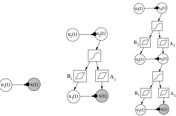
5.3 A Hierarchical Variance Model

A

u(t) s(t)

x(t) A

s(t)

x(t)

Figure 6: Model structures for linear factor analysis (FA) (left) and independent factor analysis (IFA) (right).

The final rightmost variance model in Fig. 7 is somewhat involved in that it contains both non-linearities and hierarchical modelling of variances. Before going into its mathematical details and into the two simpler models in Fig. 7, we point out that we have considered in our earlier papers related but simpler block models. In Valpola et al. (2003c), a hierarchical nonlinear model for the data x(t)is discussed without modelling the variance. Such a model can be applied for example to nonlinear ICA or blind source separation. Experimental results (Valpola et al., 2003c) show that this block model performs adequately in the nonlinear BSS problem, even though the results are slightly poorer than for our earlier computationally more demanding model (Lappalainen and Honkela, 2000; Valpola et al., 2003b; Honkela and Valpola, 2005) with multiple computational paths.

In another paper (Valpola et al., 2004), we have considered hierarchical modelling of variance using the block approach without nonlinearities. Experimental results on biomedical MEG (mag-netoencephalography) data demonstrate the usefulness of hierarchical modelling of variances and existence of variance sources in real-world data.

Learning starts from the simple structure shown in the left subfigure of Fig. 7. There a variance source is attached to each Gaussian observation node. The nodes represent vectors, with u1(t)being the output vector of the variance source and x(t)the tthobservation (data) vector. The vectors u1(t) and x(t) have the same dimension, and each component of the variance vector u1(t) models the variance of the respective component of the observation vector x(t).

Mathematically, this simple first model obeys the equations

x(t) =a1+nx(t), (28)

u1(t) =b1+nu1(t). (29)

Here the vectors a1 and b1 denote the constant means (bias terms) of the data vector x(t) and the variance variable vector u1(t), respectively. The additive “noise” vector nx(t) determines the variances of the components of x(t). It has a Gaussian distribution with a zero mean and variance exp[−u1(t)]:

A₁

1

B x(t)

x(t) u (t)

u (t)

u (t) s (t)

1

2 2

1

2

1 1

2

u (t) B

B A

A u (t)

2

u (t)

s (t)₂ s (t)₃

x(t)

1 3

Figure 7: Construction of a hierarchical variance model in stages from simpler models. Left: In the beginning, a variance source is attached to each Gaussian observation node. The nodes represent vectors. Middle: A layer of sources with variance sources attached to them is added. They layers are connected through a nonlinearity and an affine mapping. Right: Another layer is added on the top to form the final hierarchical variance model.

vector−u1(t). Similarly,

nu1(t)∼

N

(0,exp[−v1]) (31)

where the components of the vector v1 define the variances of the zero mean Gaussian variables

nu1(t).

Consider then the intermediate model shown in the middle subfigure of Fig. 7. In this second learning stage, a layer of sources with variance sources attached to them is added. These sources are represented by the source vector s2(t), and their variances are given by the respective components of the variance vector u2(t)quite similarly as in the left subfigure. The (vector) node between the source vector s2(t) and the variance vector u1(t) represents an affine transformation with a trans-formation matrix A1including a bias term. Hence the prior mean inputted to the Gaussian variance source having the output u1(t)is of the form B1f(s2(t)) +b1, where b1is the bias vector, and f(·)is a vector of componentwise nonlinear functions (7). Quite similarly, the vector node between s2(t) and the observation vector x(t)yields as its output the affine transformation A1f(s2(t)) +a1, where

a1 is a bias vector. This in turn provides the input prior mean to the Gaussian node modelling the observation vector x(t).

The mathematical equations corresponding to the model represented graphically in the middle subfigure of Fig. 7 are:

x(t) =A1f(s2(t)) +a1+nx(t), (32)

u1(t) =B1f(s2(t)) +b1+nu1(t), (33)

s2(t) =a2+ns2(t), (34)

Compared with the simplest model (28)–(29), one can observe that the source vector s2(t)of the second (upper) layer and the associated variance vector u2(t)are of quite similar form, given in Eqs. (34)–(35). The models (32)–(33) of the data vector x(t)and the associated variance vector u1(t)in the first (bottom) layer differ from the simple first model (28)–(29) in that they contain additional terms A1f(s2(t))and B1f(s2(t)), respectively. In these terms, the nonlinear transformation f(s2(t)) of the source vector s2(t)coming from the upper layer have been multiplied by the linear mixing matrices A1 and B1. All the “noise” terms nx(t), nu1(t), ns2(t), and nu2(t) in Eqs. (32)–(35) are

modelled by similar zero mean Gaussian distributions as in Eqs. (30) and (31).

In the last stage of learning, another layer is added on the top of the network shown in the middle subfigure of Fig. 7. The resulting structure is shown in the right subfigure. The added new layer is quite similar as the layer added in the second stage. The prior variances represented by the vector u3(t)model the source vector s3(t), which is turn affects via the affine transformation

B2f(s3(t)) +b2to the mean of the mediating variance node u2(t). The source vector s3(t)provides also the prior mean of the source s2(t)via the affine transformation A2f(s3(t)) +a2.

The model equations (32)–(33) for the data vector x(t)and its associated variance vector u1(t) remain the same as in the intermediate model shown graphically in the middle subfigure of Fig. 7. Note that A1 and B1 are still updated. The model equations of the second and third layer sources

s2(t)and s3(t)as well as their respective variance vectors u2(t)and u3(t)in the rightmost subfigure of Fig. 7 are given by

s2(t) =A2f(s3(t)) +a2+ns2(t), u2(t) =B2f(s3(t)) +b2+nu2(t),

s3(t) =a3+ns3(t), u3(t) =b3+nu3(t).

Again, the vectors a2, b2, a3, and b3represent the constant means (biases) in their respective models, and A2and B2 are mixing matrices with matching dimensions. The vectors ns2(t), nu2(t), ns3(t),

and nu3(t)have similar zero mean Gaussian distributions as in Eqs. (30) and (31).

It should be noted that in the resulting network the number of scalar-valued nodes (size of the layers) can be different for different layers. Additional layers could be appended in the same manner. The final network of the right subfigure in Fig. 7 uses variance nodes in building a hierarchical model for both the means and variances. Without the variance sources the model would correspond to a nonlinear model with latent variables in the hidden layer. As already mentioned, we have considered such a nonlinear hierarchical model in Valpola et al. (2003c). Note that as latent variables of the upper layer are connected to observations through multiple hidden nodes, having computation nodes as hidden nodes would result in multiple computational paths. This type of structure was used in Lappalainen and Honkela (2000), and it has a quadratic computational complexity as opposed to linear one of the networks in Figure 7.

5.4 Linear Dynamic Models for the Sources and Variances

Sometimes it is useful to complement the linear factor analysis model

x(t) =As(t) +a+nx(t) (36)

with a recursive one-step prediction model for the source vector s(t):

−1

z

A B

s(t)

x(t)

−1

z

A B

u(t) s(t)

x(t)

−1

z

−1

z

A

u(t) s(t)

x(t) C

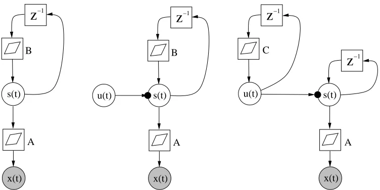
Figure 8: Three model structures. A linear Gaussian state-space model (left); the same model com-plemented with a super-Gaussian innovation process for the sources (middle); and a dy-namic model for the variances of the sources which also have a recurrent dydy-namic model (right).

The noise term ns(t)is called the innovation process. The dynamic model of the type (36), (37) is used for example in Kalman filtering (Haykin, 1998, 2001), but other estimation algorithms can be applied as well (Haykin, 1998). The left subfigure in Fig. 8 depicts the structure arising from Eqs. (36) and (37), built from the blocks.

A straightforward extension is to use variance sources for the sources to make the innovation process super-Gaussian. The variance signal u(t) characterises the innovation process of s(t), in effect telling how much the signal differs from the predicted one but not in which direction it is changing. The graphical model of this extension is depicted in the middle subfigure of Fig. 8. The mathematical equations describing this model can be written in a similar manner as for the hierarchical variance models in the previous subsection.

Another extension is to model the variance sources dynamically by using one-step recursive prediction model for them:

u(t) =Cu(t−1) +c+nu(t).

This model is depicted graphically in the rightmost subfigure of Fig. 8. In context with it, we use the simplest possible identity dynamical mapping for s(t):

s(t) =s(t−1) +ns(t).

The latter two models introduced in this subsection will be tested experimentally later on in this paper.

5.5 Hierarchical Priors

ai j of a mixing matrix A can be defined via the Gaussian distributions

p(ai j|vai) =

N

(ai j; 0,exp(−vai)),

p(va_i |mva,vva) =

N

(va_i; mva,exp(−vva)).

Finally, the priors of the quantities mva and vva have flat Gaussian distributions

N

(·; 0,100)

(the constants depending on the scale of the data). When going up in the hierarchy, we use the same distribution for each column of a matrix and for each component of a vector. On the top, the number of required constant priors is small. Thus very little information is provided and needed a priori. This kind of hierarchical priors are used in the experiments later on this paper.

6. Learning

Let us now discuss the overall learning procedure, describing also briefly how problems related with learning can be handled.

6.1 Updating of the Network

The nodes of the network communicate with their parents and children by providing certain expec-tations in the feedforward direction (from parents to children) and gradients of the cost function with respect to the same expectations in the feedback direction (from children to parents). These expectations and gradients are summarised in Tables 1 and 2.

The basic element for updating the network is the update of a single node assuming the rest of the network fixed. For computation nodes this is simple: each time when a child node asks for expectations and they are out of date, the computational node asks from its parents for their expectations and updates its own ones. And vice versa: when parents ask for gradients and they are out of date, the node asks from its children for the gradients and updates its own ones. These updates have analytical formulas given in Section 4.

For a variable node to be updated, the input expectations and output gradients need to be up-to-date. The posterior approximation q(s) can then be adjusted to minimise the cost function as explained in Section 4. The minimisation is either analytical or iterative, depending on the situation. Signals propagating outwards from the node (the output expectations and the input gradients) of a variable node are functions of q(s)and are thus updated in the process. Each update is guaranteed not to increase the cost function.

One sweep of updating means updating each node once. The order in which this is done is not critical for the system to work. It would not be useful to update a variable twice without updating some of its neighbours in between, but that does not happen with any ordering when updates are done in sweeps. We have used an ordering where each variable node is updated only after all of its descendants have been updated. Basically when a variable node is updated, its input gradients and output expectations are labelled as outdated and they are updated only when another node asks for that information.

Learning a model typically takes thousands of sweeps before convergence. The cost function decreases monotonically after every update. Typically this decrease gets smaller with time, but not always monotonically. Therefore care should be taken in selecting the stopping criterion. We have chosen to stop the learning process when the decrease in the cost during the previous 200 sweeps is lower than some predefined threshold.

6.2 Structural Learning and Local Minima

The chosen model has a pre-specified structure which, however, has some flexibility. The number of nodes is not fixed in advance, but their optimal number is estimated using variational Bayesian learning, and unnecessary connections can be pruned away.

A factorial posterior approximation, which is used in this paper, often leads to automatic prun-ing of some of the connections in the model. When there is not enough data to estimate all the parameters, some directions remain ill-determined. This causes the posterior distribution along those directions to be roughly equal to the prior distribution. In variational Bayesian learning with a factorial posterior approximation, the ill-determined directions tend to get aligned with the axes of the parameter space because then the factorial approximation is most accurate.

The pruning tendency makes it easy to use for instance sparsely connected models, because the learning algorithm automatically selects a small amount of well-determined parameters. But at the early stages of learning, pruning can be harmful, because large parts of the model can get pruned away before a sensible representation has been found. This corresponds to the situation where the learning scheme ends up into a local minimum of the cost function (MacKay, 2001). A posterior approximation which takes into account the posterior dependences has the advantage that it has far less local minima than a factorial posterior approximation. It seems that Bayesian learning algorithms which have linear time complexity cannot avoid local minima in general.

However, suitable choices of the model structure and countermeasures included in the learning scheme can alleviate the problem greatly. We have used the following means for avoiding getting stuck into local minima:

• Learning takes place in several stages, starting from simpler structures which are learned first before proceeding to more complicated hierarchic structures. An example of this technique was presented in Section 5.3.

• New parts of the network are initialised appropriately. One can use for instance principal component analysis (PCA), independent component analysis (ICA), vector quantisation, or kernel PCA (Honkela et al., 2004). The best option depends on the application. Often it is useful to try different methods and select the one providing the smallest value of the cost function for the learned model. There are two ways to handle initialisation: either to fix the sources for a while and learn the weights of the model, or to fix the weights for a while and learn the sources corresponding to the observations. The fixed variables can be released gradually (Valpola et al., 2003c, Section 5.1).

• Automatic pruning is discouraged initially by omitting the term

2Var{s2}

∂C ∂Var{s1s2}

in the multiplication nodes (Eq. (23)). This effectively means that the mean of s1is optimisti-cally adjusted as if there were no uncertainty about s2. In this way the cost function may increase at first due to overoptimism, but it may pay off later on by escaping early pruning.

• New sources si(t)(components of the source vector s(t)of a layer) are generated, and pruned sources are removed from time to time.

• The activations of the sources are reset a few times. The sources are re-adjusted to their places while keeping the mapping and other parameters fixed. This often helps if some of the sources are stuck into a local minimum.

7. Experimental Results

The Bayes Blocks software (Valpola et al., 2003a) has been applied to several problems.

Valpola et al. (2004) considered several models of variance. The main application was the analysis of MEG measurements from a human brain. In addition to features corresponding to brain activity the data contained several artifacts such as muscle activity induced by the patient biting his teeth. Linear ICA applied to the data was able to separate the original causes to some degree but still many dependencies remained between the sources. Hence an additional layer of so-called variance sources was used to find correlations between the variances of the innovation processes of the ordinary sources. These were able to capture phenomena related to the biting artifact as well as to rhythmic activity.

An astrophysical problem of separating young and old star populations from a set of elliptical galaxy spectra was studied by one of the authors in Nolan et al. (2006). Since the observed quantities were energies and thus positive and since the mixing process was also known to be positive, it was necessary for the subsequent astrophysical analysis to be feasible to include these constraints to the model as well. The standard technique of putting a positive prior on the sources was found to have the unfortunate technical shortcoming of inducing sparsely distributed factors, which was deemed inappropriate in that specific application. To get rid of the induced sparsity but to still keep the positivity constraint, the nonnegativity was forced by rectification nonlinearities (Harva and Kab´an, 2007). In addition to finding an astrophysically meaningful factorisation, several other specifications were needed to be met related to handling of missing values, measurements errors and predictive capabilities of the model.

In Raiko (2005), a nonlinear model for relational data was applied to the analysis of the board game Go. The difficult part of the game state evaluation is to determine which groups of stones are likely to get captured. A model similar to the one that will be described in Section 7.2, was built for features of pairs of groups, including the probability of getting captured. When a learned model is applied to new game states, the estimates propagate through a network of such pairs. The structure of the network is thus determined by the game state. The approach can be used for inference in relational databases.

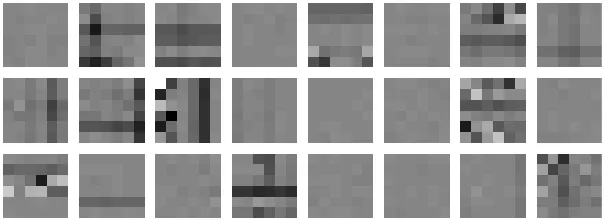
Figure 9: Samples from the 1000 image patches used in the extended bars problem. The bars include both standard and variance bars in horizontal and vertical directions. For instance, the patch at the bottom left corner shows the activation of a standard horizontal bar above the horizontal variance bar in the middle.

7.1 Bars Problem

The first experimental problem studied was testing of the hierarchical nonlinear variance model in Figure 7 in an extension of the well-known bars problem (Dayan and Zemel, 1995). The data set consisted of 1000 image patches each having 6×6 pixels. They contained both horizontal and vertical bars. In addition to the regular bars, the problem was extended to include horizontal and vertical variance bars, characterised and manifested by their higher variance. Samples of the image patches used are shown in Figure 9.

The data were generated by first choosing whether vertical, horizontal, both, or neither orienta-tions were active, each with probability 1/4. Whenever an orientation is active, there is a probability 1/3 for a bar in each row or column to be active. For both orientations, there are 6 regular bars, one for each row or column, and 3 variance bars which are 2 rows or columns wide. The intensities (grey level values) of the bars were drawn from a normalised positive exponential distribution having the pdf p(z) = exp(−z),z≥0, p(z) = 0,z<0. Regular bars are additive, and variance bars produce additive Gaussian noise having the standard deviation of its intensity. Finally, Gaussian noise with a standard deviation 0.1 was added to each pixel.

weight matrices is depicted as a pixel with the appropriate grey level value in Fig. 10. The pixels of A2 and B2 are ordered similarly as the patches of A1 and B1, that is, vertical bars on the left and horizontal bars on the right. Regular bars, present in the mixing matrix A1, are reconstructed accurately, but the variance bars in the mixing matrix B1 exhibit some noise. The grouping of horizontal and vertical orientations is clearly visible in the mixing matrix A2. For instance, the first patch in A2 has non-zero (black) weights to all the vertical features, that is, left side pixels in A2 activate sources corresponding to the left side patches in A1and B1.

A2(18×2) B2(18×2)

A1(36×18) B1(36×18)

Figure 10: Results of the extended bars problem: Posterior means of the weight matrices after learning. The sources of the second layer have been ordered for visualisation purposes according to the weight (mixing) matrices A2 and B2. The elements of the matrices have been depicted as pixels having corresponding grey level values. The 18 pixels in the weight matrices A2and B2 correspond to the 18 patches in the weight matrices A1 and B1.

A comparison experiment with a simplified learning procedure was run to demonstrate the im-portance of local optima. The creation and pruning of layers were done as before, but other methods for avoiding local minima (addition of nodes, discouraging pruning and resetting of sources) were disabled. The resulting weights can be seen in Figure 11. This time the learning ends up in a subop-timal local optimum of the cost function. One of the bars was not found (second horizontal bar from the bottom), some were mixed up in a same source (most variance bars share a source with a regular bar), fourth vertical bar from the left appears twice, and one of the sources just suppresses variance everywhere. The resulting cost function (4) is worse by 5292 compared to the main experiment. The ratio of the model evidences is thus roughly exp(5292).

po-0 500 1000 1500 1

1.5 2 2.5 3 3.5

4x 10

4

A2(14×2) B2(14×2)

A1(36×14) B1(36×14)

Figure 11: Left: Cost function plotted against the number of learning sweeps. Solid curve is the main experiment and the dashed curve is the comparison experiment. The peaks appear when nodes are added. Right: The resulting weights in the comparison experiment are plotted like in Figure 10.

prior likelihood posterior approximation

Figure 12: A typical example illustrating the posterior approximation of a variance source.

tential given its children (the first component of x(1)). Assuming the posteriors of other variables accurate, we can plot the true posterior of this variable and compare it to the Gaussian posterior approximation. Their difference is only 0.007 measured by Kullback-Leibler divergence.

7.2 Missing Values in Speech Spectra

In hierarchical nonlinear factor analysis (HNFA) (Valpola et al., 2003c), there are a number of layers of Gaussian variables, the bottom-most layer corresponding to the data. There is a nonlinearity and a linear mixture mapping from each layer to all the layers below it.

HNFA resembles the model structure in Section 5.3. The model structure is depicted in the left subfigure of Fig. 13. Model equations are

h(t) =As(t) +a+nh(t),