Cost Allocation of Operational Materials for an Alloy and Special Steel Plant using Excel Solver

ISSN: 2306-9007 Aljasser, Sasidhar & Toppur (2014) 1145

I

I

R

M

B

R

V

R

M

B

R

Cost Allocation of Operational Materials for an Alloy and

Special Steel Plant using Excel Solver

IBRAHIM ABDULLAH ALJASSER

Quantitative Analysis Department, College of Business Administration King Saud University, Riyadh, Kingdom of Saudi Arabia

Email: [email protected]

BOKKASAM SASIDHAR

Quantitative Analysis Department, College of Business Administration King Saud University, Riyadh, Kingdom of Saudi Arabia

Email: [email protected]; [email protected]

BADRI TOPPUR

Operations Management Department, Great Lakes Institute of Management, Thiruvanmiyur, Chennai 600041. India

Email: [email protected]

Abstract

While manufacturing different grades of steel in an alloy and special steel plant, it is practically impossible to allocate the cost of major operational materials such as refractories, electrodes and nipples, ingot moulds etc. to each grade of steel. Conventionally, cost allocation of operational materials is done based on the time taken for processing a particular grade of steel. A more accurate picture of the utilization levels of these operational materials by different grades of steel can be obtained if one factors in the differences in the rate of consumption, in view of the variations in temperature and intensity of chemical reactions. Earlier quadratic model with a non-linear objective function and linear constraints has been envisaged to estimate the consumption pattern for each grade manufactured, so that a realistic grade-wise cost can be arrived at. In this paper, use of Excel Solver has been demonstrated based on the quadratic model envisaged earlier. The same has been validated with results obtained using examples, which the managers will be able to use for obtaining the results immediately for scaled-up scenarios.

Key Words: Cost allocation, Operational Materials, Steel, Mathematical Modeling, Quadratic Programming, Excel, Solver.

Introduction

ISSN: 2306-9007 Aljasser, Sasidhar & Toppur (2014) 1146

I

I

R

M

B

R

V

R

M

B

R

allocation needs to be made among the different grades of steel that are made during a campaign. The grade-wise costing is typically done in four stages; cost sheet for hot metal, cost sheet for melting shop, cost sheet for conditioning, and cost sheet for each of the mills. The cost at the end of one stage is considered as the input cost for the next stage. The present paper focuses its attention in arriving at the grade-wise cost at the melting shop.

Total Cost at the melting shop is the sum of the direct variable cost and the process cost. Direct variable cost components include all the raw and operational materials which can be directly allocated to a particular steel grade without any ambiguity. However, operational materials such as refractories, electrodes and nipples, ingot moulds, power, oxygen, shops and foundry etc. get consumed continuously while manufacturing all grades of steel. Hence segregation of the cost of these operational materials for individual grades poses a challenge. Conventionally, cost allocation of these operational materials is being done based on the time taken for processing a particular grade of steel. An average cost per unit time is calculated irrespective of the grades of steel manufactured. Based on the grade-wise time consumption, proportionate allocation of total cost is effected. However, this procedure is not quite satisfactory, as the consumption of operational materials not only depend on the time but also the grade of steel manufactured. Shaw (1972) discusses the types of refractories needed for various furnace-sections, which have been well established. Turkdogan (1983) elaborates the complex relationships between the wear of the refractory linings and the content of iron oxides, calcium oxide, silica, phosphorus, alumina in the slag, temperature and dissolution of refractory oxides of alumina, lime, magnesia in the molten. Similarly, the factors having effect on electrodes during usage in the arc furnaces, such as the mechanical shocks during melt-down, oxidation, thermal shocks, current density and electrical resistivity at the nipple joint have been elaborated by Singh and Prasad (1982). Since the consumption of operational materials vary from one grade to another, consideration of only production time for the allocation of cost is not entirely satisfactory.

Sasidhar and Achary (1991) have envisaged a quadratic model with a non-linear objective function and linear constraints to estimate the consumption pattern for each quality manufactured. The same problem was attacked using the Particle Swarm algorithm by Ahmad et al. (2012). In this paper, the quadratic modeling of costing method has been automated on Excel worksheets by applying solver. This costing utility will bring in modifications and enhancements that will accommodate other plant realities and complexities.

Model Development

Sasidhar and Achary (1991) indicated that a more realistic cost accounting for operational materials is the one that considers the differing rates of consumption of the operational materials for different grades. This concept was formulated as a quadratic programming model by phrasing the variables so that the constraints in this problem could be stated in the standard form of mathematical programming: Ax = b.

Towards this end the following variables were defined:

• Let xj , j = 1, 2,…,n denote the quantum of the operational material consumed per ton of

production of steel grade j.

• Let bi, i = 1, 2, …,m denote the quantity of the operational material consumed during the ith

campaign. If the quantity bi is taken to be one, then xj denotes the fraction of material consumed

instead of quantum.

• Let aij, i = 1, 2, …, m; j = 1, 2, …, n denote the quantum of production of grade j steel in campaign

i

Let A = [aij] denote the matrix of campaign-wise and grade-wise production quantities. The term Ax is now

ISSN: 2306-9007 Aljasser, Sasidhar & Toppur (2014) 1147

I

I

R

M

B

R

V

R

M

B

R

xj is strictly positive as it denotes the quantity of material consumed per ton of production of grade j steel.

Given these variables and matrix definitions, the problem is to solve a system of linear equations of the form:

Ax = b x > 0

Inverting A and multiplying the result with b does not guarantee x > 0, because A-1b may have zero entries. Direct application of Linear Programming will also indicate infeasibility; this is because a basic feasible solution obtained in LP will have many variables at value zero, and we have demanded positive x values. One alternative to these methods is to minimize squared difference or to minimize absolute difference between left-hand-side and right-hand-side of Ax=b. Taking the “squared difference” approach leads to a quadratic objective function:

Minimize:

Subject to the constraint that all the consumption levels are strictly positive xj > 0 for all j = 1, 2, …, n. The

objective function above was shown through matrix multiplication to be equivalent to the objective function below:

Maximize:

The advantage of this transformation is that any specialized algorithm that is available for a quadratic programming can be used. To enforce the constraint of strictly positive xj, a sufficiently small lower bound

value Є can be used. In this paper, the quadratic modeling of costing method has been automated on Excel worksheets by applying solver. Also, the effect of changes in fixing the lower bound value Є for the variables has been identified to arrive at an optimal value for Є.

Illustrative Examples

Example 1

The illustrative example 1 with two qualities and three campaigns, as considered by Sasidhar and Achary (1991) is given in Table 1.

Table 1: Production and duration details for three campaigns

Campaign Stainless Steel Tool Steel Total

Production (tons) (000s) Duration (hrs) Production (tons) (000s) Duration (hrs) Production (tons) (000s) Duration (hrs)

1 1 172 3 452 4 624

2 2 312 1 156 3 468

3 3 460 0.5 86 3.5 546

Total 6 944 4.5 694 10.5 1638

Let xj , j = 1, 2 denote the quantum of the operational material consumed per ton of production of stainless

steel and tool steel grades respectively.

 

















ij

x

b

a

Z

b

2A

p

and

A

2A

c

where

2

1

*











b

b

cx

x

x

p

ISSN: 2306-9007 Aljasser, Sasidhar & Toppur (2014) 1148

I

I

R

M

B

R

V

R

M

B

R

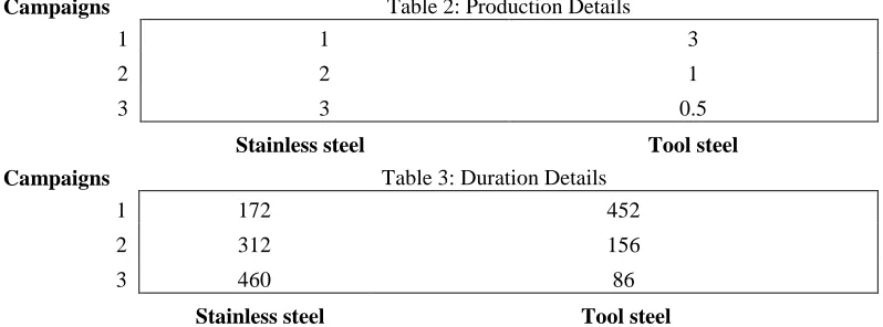
The excel inputs for production and duration details of the problem are shown in Tables 2 and 3.

Campaigns Table 3: Duration Details

1 172 452

2 312 156

3 460 86

Stainless steel Tool steel

Considering the lower bound of each variable as 0.0001 and by applying the solver, we obtain the solution as in Table 4.

Table 4: Solver solution for Example 1

Consumption of Refractory per ton of each grade Objective Function

0.3185179 0.237036917 2.977777778

X Constrained to be positive

0.3185179 >= 0.0001

0.237036917 >= 0.0001

For the problem scenario described in Table 1, by using solver, we obtain x1 = 0.3185 and x2 = 0.2370.

Thus stainless steel consumes 1.3439 times more refractory material than tool steel. This fact is not revealed in the time-based costing method. We can encode this fact by the equality:

1.3439x1 = x2

Setting 6000(1.3439x2) + 4500x2= Rs. 1200,000

This inequality in cost allocation is a much more faithful reflection of the actual consumption rate of refractory material per ton of stainless steel and tool steel. We have achieved with the computer program, the same solution as obtained in the paper. It can be observed that the methodology adopted will involve the quantities of each grade of steel produced and the cost of the material per campaign. It can be noted that this procedure does not involve the production durations for various grades.

Using the computer program, large problems can be solved in a similar way, involving many grades of steel and operational materials in different campaigns. The solution of one large example involving refractory and electrodes for seven grades of steel is shown as an incremental advance to the work. At the click of a button, the application performs various transposes and products using matrix multiplication, after obtaining the production data from the user.

Example 2

Consider the data in Table 5 which displays Production data for a scenario of seven grades of steel and five refractory campaigns.

Campaigns

Table 2: Production Details

1 1 3

2 2 1

3 3 0.5

ISSN: 2306-9007 Aljasser, Sasidhar & Toppur (2014) 1149

I

I

R

M

B

R

V

R

M

B

R

Table 5: Production details for five campaigns of refractory

PRODUCTION

DETAILS Steel Grades

1 2 3 4 5 6 7 Total

Refractory Campaigns

1 1 3 2 2 1 3 4 16

2 2 1 1 4 3 2 5 18

3 3 0.5 2.5 2 2.5 4 1 15.5

4 2 1 2 1 3 1 2 12

5 1 0.5 2.4 3 2 1 3 12.9

Total 9 6 9.9 12 11.5 11 15 74.4

In order to identify the effect of changes in the solution for different values of the lower bound value Є for the variables, different values of Є have been considered and by applying the excel solver, we obtain the solution as in Table 6.

Table 6: Solver solution for refractory consumption of Example 2 for different values of Є

Є X1 X2 X3 X4 X5 X6 X7

0.1 0.1 0.1 0.1 0.1 0.1 0.1 0.1

0.01 0.01 0.05599 0.20903 0.01 0.12208 0.01 0.05805

0.001 0.02387 0.05982 0.21174 0.01199 0.11314 0.001 0.05825

0.0001 0.00956 0.05671 0.21063 0.00911 0.12297 0.00808 0.05839

0.00001 0.00956 0.05671 0.21063 0.00911 0.12297 0.00808 0.05839

0.000001 0.00956 0.05671 0.21063 0.00911 0.12297 0.00808 0.05839

It can be observed that, as we consider smaller values for Є, the values for the solution converge to a limiting value. It can be observed that the solution vector remains the same for values of Є ≤ 0.0001. Hence, we can consider the optimal value of Є to be 0.0001.

Considering Є=0.0001, the problem of Example 2 has been solved. The excel output for problem is shown in Table 7.

Table 7: Solver solution for refractory consumption of Example 2 x-vector

0.009560654 0.056711071 0.210630564 0.009117617 0.122969952 0.008081846 0.058398428 x

constrained to be

positive

0.009560654 >= 0.0001

0.056711071 >= 0.0001 5.931714589

0.210630564 >= 0.0001 22.03097872

0.009117617 >= 0.0001 0.953660362

0.122969952 >= 0.0001 12.86208582

0.008081846 >= 0.0001 0.84532355

0.058398428 >= 0.0001 6.108204341

Objective function value

ISSN: 2306-9007 Aljasser, Sasidhar & Toppur (2014) 1150

I

I

R

M

B

R

V

R

M

B

R

Using the solver we can obtain the following values of x

x1= 0.009560654 x2=0.056711071 x3=0.210630564 x4 =0.009117617

x5=0.122969952 x6=0.008081846 x7=0.058398428

We can convert all these levels to x1 terms using the ratios.

x2 =5.93171x1 x3 = 22.03098x1 x4 = 0.95366x1 x5=12.86209x1

x6=0.84532x1 x7 = 6.10820x1

We can then multiply these ratios by the tonnage per grade of steel and set it equal to the total campaign cost k, thereby obtaining the cost per ton for each grade of steel.

9000(x1) + 6000(5.93171x1) + 9900(22.03098x1) +12000(0.95366x1) +11500(12.86209x1) +

11000(0.84532x1) + 15000(6.10820x1) = k

Conclusion

In this paper, a working implementation of the non-linear program using excel solver is presented. The procedure has been validated with results obtained and this enables the managers to solve large problems involving many grades of steel and operational material campaigns. The same technique can be used to determine the consumption pattern of all such operational materials for arriving at a realistic grade-wise cost. In future the plant managers will be able to use the excel solver for obtaining the results immediately for scaled-up scenarios.

Acknowledgement

This paper is supported by the Research Center at the College of Business Administration and the Deanship of Scientific Research at King Saud University, Riyadh.

References

Ahmad Al Hammad, Mahmoud M. El-Sherbiny & Bokkasam Sasidhar (2012). Particle swarm algorithm

for cost allocation of major operational materials in an alloy steel plant. African Journal of Business

Management, 6(11), 3851-3855.

Sasidhar, B & Achary, K..K. (1991). Applications of O.R. techniques in cost allocation of major operational materials in an alloy and special steel manufacturing unit. International Journal of Production Economics, 22, 189-193

Shaw, K.. (1972). Refractories and Their Uses. Applied Science Publishers, London.

Singh, B. P. & Prasad, L. (1982). Graphite electrodes for high intensity furnaces: The Indian scene-electric steel making in the eighties: Challenges and opportunities. In: Proc. Int. Conf. organized by Steel Furnace Association of India, 246-251.

Turkdogan, E. T. (1983). Physicochemical Properties of Molten Slags and Glasses. The Metals Society, London.