Supervised Learning via Euler’s Elastica Models
Tong Lin [email protected]
Hanlin Xue [email protected]
Ling Wang [email protected]
Bo Huang [email protected]
Hongbin Zha [email protected]
Key Laboratory of Machine Perception (Ministry of Education) School of Electronics Engineering and Computer Science Peking University, Beijing, 100871, China
Editor:Mikhail Belkin
Abstract
This paper investigates the Euler’s elastica (EE) model for high-dimensional supervised learning problems in a function approximation framework. In 1744 Euler introduced the elastica energy for a 2D curve on modeling torsion-free thin elastic rods. Together with its degenerate form of total variation (TV), Euler’s elastica has been successfully applied to low-dimensional data processing such as image denoising and image inpainting in the last two decades. Our motivation is to apply Euler’s elastica to high-dimensional super-vised learning problems. To this end, a supersuper-vised learning problem is modeled as an energy functional minimization under a new geometric regularization scheme, where the energy is composed of a squared loss and an elastica penalty. The elastica penalty aims at regularizing the approximated function by heavily penalizing large gradients and high curvature values on all level curves. We take a computational PDE approach to minimize the energy functional. By using variational principles, the energy minimization problem is transformed into an Euler-Lagrange PDE. However, this PDE is usually high-dimensional and can not be directly handled by common low-dimensional solvers. To circumvent this difficulty, we use radial basis functions (RBF) to approximate the target function, which reduces the optimization problem to finding the linear coefficients of these basis functions. Some theoretical properties of this new model, including the existence and uniqueness of so-lutions and universal consistency, are analyzed. Extensive experiments have demonstrated the effectiveness of the proposed model for binary classification, multi-class classification, and regression tasks.
“Read Euler, read Euler, he is our master in everything” — Pierre-Simon Laplace (1749–1827)
1. Introduction
Supervised learning (Murphy, 2012; Hastie et al., 2009; Bishop, 2006) aims at inferring a function that maps inputs to desired outputs under the guidance of training data. Two main tasks in supervised learning are classification and regression. Numerous supervised learn-ing methods have been developed in several decades; Caruana and Niculescu-Mizil (2006) gave a comprehensive empirical comparison of these methods. A most recent evaluation of classification methods was conducted by Fern´andez-Delgado et al. (2014): 179 classifiers arising from 17 families were compared on 121 data sets, showing that random forests, sup-port vector machines (SVM), neural networks, and boosting are among the top methods nowadays. Roughly speaking, existing methods can be divided into two main categories: statistics based and function learning based. One advantage of function learning methods is that powerful mathematical theories in functional analysis can be explored rather than doing optimizations on discrete data points.
Most function learning methods can be derived from the energy regularization frame-work, which minimizes a fitting loss term plus a smoothing penalty. It is arguable that the most successful classification and regression method is the support vector machines (SVM) (Vapnik, 1998; Cristianini and Shawe-Taylor, 2000; Sch¨olkopf and Smola, 2002), whose cost function is composed of a hinge loss and a RKHS norm penalty determined by a kernel. There are several variants of SVM by combining different losses and different penalties (Steinwart, 2005; Bartlett et al., March 2006; Huang et al., 2014). In particular, when replacing the hinge loss by a squared loss, the modified algorithm is called Regular-ized Least Squares (RLS) method (Rifkin, 2002). Instead of considering a variety of loss terms, manifold regularization (Belkin et al., 2006) introduced a geometric regularizer of squared gradient magnitude on a manifold. Its discrete version corresponds to graph Lapla-cian regularization (Zhou and Sch¨olkopf, 2005; Nadler et al., 2009). A most recent work is the geometric level set (GLS) classifier (Varshney and Willsky, 2010), with an energy functional composed of a margin-based loss and a geometric regularization term based on the surface area of the decision boundary. The GLS classifier was motivated by the study of minimal surfaces and its applications in image processing. Experiments showed that GLS is competitive with SVM and other state-of-the-art classifiers.
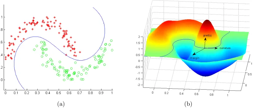
(a) (b)
Figure 1: Results on two moon data by using the EE classifier. (a) Decision boundary (in blue) that separates two classes of points (represented by red stars or green circles); (b) learned target function illustrated as a surface in a 3D space.
benchmark data sets against state-of-the-art methods. Figure 1 shows the classification result and the learned target function on the popular example of two moon dataset by using the EE classifier. Note that three important factors considered in the EE classifier, gradient, curvature, and margin between two classes, are depicted in different directions on one data point of the produced decision boundary in Figure 1(b).
Although some researchers in the machine learning community may think that the super-vised learning problems have been widely studied and several leading algorithms like SVM (Vapnik, 1998; Cristianini and Shawe-Taylor, 2000; Sch¨olkopf and Smola, 2002), boosting (Schapire and Freund, 2012), and random forests (Breiman, 2001) have been available to achieve superb classification performance, we argue that this work provides a new perspec-tive on understanding supervised learning problems. Particularly, the contributions of this paper are:
the squared loss is equivalent to a margin-based loss (1−yf(x))2, called the quadratic loss (Bartlett et al., March 2006, table 1), sincey∈ {−1,+1}in binary classifications. On the other hand, the term gradient is related to the slope of function values in a continuous setting, while the curvature measures the degree to which all the level curves (including the decision boundary) is curved. Both gradients and curvatures are geometric measurements that reflect the complexity of the output classifier. The trade-off between the squared loss and the complexity involving gradients and curvatures in this work is new to the machine learning community.
2. Euler-Lagrange PDEs that characterize the optimal solution for supervised learning problems. Historically, PDEs have been used to describe a wide range of physical phe-nomena such as sound, heat, fluid flow, electrostatics, electrodynamics, or elasticity. Surprisingly, these seemingly distinct physical phenomena can be unified under a PDE framework, which implies that they are essentially governed by same or similar na-ture’s mechanism. A natural question is, can PDEs be applicable to high-dimensional supervised learning problems? To the best of our knowledge, Varshney and Will-sky (2010) were the first attempt to propose level set based PDEs for classification. Following this research line, we propose the Euler-Lagrange PDEs derived from Eu-ler’s elastica model and its degenerate total-variation model, for classification and regression. These PDEs reveal equilibrium conditions of the desired fitting process for supervised learning.
3. Two numerical algorithms for solving the elastica based supervised learning problem in high dimensions. By using radial basis function approximation, we present two PDE solvers: the gradient descent time marching method and the lagged linear equation iteration method.
The remainder of this paper is organized as follows. In Section 2 we begin with a brief review of TV and EE models used in image processing. The proposed models for supervised learning are described in Section 3, followed by the corresponding numerical solutions presented in Section 4. Some theoretical properties of the proposed models are discussed in Section 5. Section 6 presents the experimental results, and Section 7 concludes the paper.
2. Preliminaries
For better understanding the proposed method, we firstly review the notions of total vari-ation and Euler’s elastica from an image processing perspective, and point out some con-nections with prior work in the machine learning literature.
2.1 Total Variation (TV)
interval [a, b]∈Ris the quantity
Vba(f) = sup
P nP−1
X
i=0
|f(xi+1)−f(xi)|, (1)
where the supremum runs over the set of all partitionsP of the given interval [a, b], withnP
being the number of points in a specific partitionP. Iff is differentiable and its derivative is Riemann-integrable, the total variation can be written as
Vba(f) = Z b
a
|f0(x)|dx.
Intuitively it measures the total distance along the direction of the y-axis, neglecting the contribution of motion along x-axis, traveled by a point moving along the graph. Notice that if f0(x) > 0 for all x ∈ [a, b], it is simply equal to f(b)−f(a) by the fundamental theorem of calculus.
The modern definition is based on the concept of distributional derivatives. Let Ω⊂R be a bounded open interval. A functionf ∈L1(Ω) is said to be of bounded variation (BV) if
sup
ϕ
nZ
Ω
f(x)ϕ0(x)dx:ϕ∈Cc1(Ω),kϕkL∞(Ω) <1 o
<∞, (2)
where Cc1(Ω) is the space of continuously differentiable functions with compact support in Ω, and k · kL∞(Ω) is the essential supremum norm. Note that this definition may have some variants, e.g. imposing the test function that satisfies ϕ∈Cc∞(Ω) and kϕkC0(Ω) <1
(Golubov and Vitushkin, 2001). An equivalent definition is that BV functions are functions whose distributional derivative is a finite Radon measure. Also the two definitions (1) and (2) are consistent. It is natural to generalize the definition (2) for functions of several variables. For an open Ω⊂Rd, the total variation of f ∈L1(Ω) is given by
sup
ϕ
nZ
Ω
f∇ ·ϕ dx:ϕ= (ϕ1, ϕ2,· · ·, ϕd)∈Cc1(Ω, Rd),kϕkL∞(Ω)<1 o
<∞, (3)
whereϕis a vector-valued test function, ∇ ·ϕ=P
∂ϕi/∂xi is the divergence operator, and
all the components ofϕhas aL∞(Ω)-norm less than one. For more details of TV definitions and the BV function space, one can refer to Chan and Shen (2005), Aubert and Kornprobst (2006), Ambrosio et al. (2000), Giusti (1994), and Golubov and Vitushkin (2001).
By penalizing large gradients of the target functions, total variation has been widely used for image processing tasks such as denoising and inpainting. The pioneering work is Rudin, Osher, and Fatemi’s image denoising model (Rudin et al., 1992):
E[u] = Z
Ω
(u−u0)2+λ|∇u|dx,
is a p-Sobolev regularization term (p = 1) where the gradient ∇u is understood in the distributional sense. The main benefit is to preserve significant image edges during the denoising procedure (Chan and Shen, 2005; Aubert and Kornprobst, 2006), as image edges are important features that should be faithfully retained in image processing. The common downside of TV-based methods is that piecewise constant images with |∇u| = 0 almost everywhere are favored over piecewise smooth images, which is the so-called staircasing effect (Duan et al., 2013). Euler’s elastica model is one of high order approaches to overcome this drawback, which is described in the next subsection.
In the machine learning literature, p-Sobolev regularizer can be found in the literature of nonparametric smoothing splines, generalized additive models, and projection pursuit regression models (Hastie et al., 2009). Specifically, Belkin et al. (2006) proposed the manifold regularization term
Z
x∈M
|∇Mu|2dx,
for any smooth functionu(x) on a manifoldM. On the other hand, discrete graph Laplacian regularization was discussed in Zhou and Sch¨olkopf (2005) as
X
v∈V
|∇vu|p,
wherevis a vertex from a vertex setV, andpis an arbitrary number. This penalty measures the roughness of the discrete function u over a graph.
2.2 Euler’s Elastica (EE)
The elastica energy first appeared in Euler’s work in 1744 on modeling torsion-free thin elastic rods (for the history see Levien, 2008; Fraser, 1991). Then Mumford (1994) rein-troduced elastica into computer vision for measuring the quality of interpolating curves in disocclusion. Later, elastica based image inpainting methods were developed in Masnou and Morel (1998) and Chan et al. (2002).
A smooth curve γ is said to be Euler’s elastica if it is the equilibrium curve of the elasticity energy:
E[γ] = Z
γ
(a+bκ2)ds, (4) where a and b are two non-negative constant weights, κ denotes the scalar curvature (see Appendix A for its definition), anddsis an infinitesimal arc length element. Euler obtained the energy in studying the steady shape of a thin and torsion-free rod under external forces. The curve implies the lowest elastica energy, thus getting its name. The ratioa/b(ifb6= 0) indicates the relative importance of the total length versus total squared curvature (Chan and Shen, 2005, chap. 2.1).
is an interesting Bayesian rationale revealed by Mumford (1994) (see also Chan et al., 2002) by considering the random walk of a drunk. Suppose the drunk starts from the origin of a 2-D ground and each step is straight. With some distribution assumptions on the step size and the orientation of each step, the maximum likelihood estimation (MLE) of such discrete random walk is approximately equivalent to the minimization of the elastica energy (4) in a continuous fashion. This drunk walking model also sheds light on the choice of “2” for the curvature power in (4). For anyp >1, one could consider the generalp-elastica energy
Ep[γ] =
Z
γ
(a+b|κ|p)ds.
Notice that the situation of p= 1 is less ideal since in this case the total curvature energy permits sudden turns. Chan et al. (2002) pointed out that generic stationary points of the p-elastica energy are forbidden when p ≥ 3, implying that p ∈(1,3) sounds to be a good choice.
A common approach to bridge the gap between a prior energy model for curves and that for images is using level sets (or called isophotes), pioneered by Osher and Sethian (1988). By “lifting” a curve prior model into a 2D space, one can construct an image prior model imposed on all the level curves of an image (corresponding to a 2D function). Formally, the Euler’s elastica of all the level curves of an image u can be expressed as
E[u] = Z L
l=0 Z
γl:u=l
(a+bκ2)dsdl, (5)
whereγl is the level curve determined byu(x) =l, and the level valuelvaries in the image
range [0, L]. Letdt denote an infinitesimal length element along the normal direction n of the level curve (or along the steepest ascent curve), then we have
dl
dt =|∇u| or dl =|∇u|dt.
Thus by the co-area formula (Giusti, 1994), the integrated elastica energy (5) now passes on to u by
E[u] = Z L
l=0 Z
γl:u=l
(a+bκ2)|∇u|dtds= Z
Ω
(a+bκ2)|∇u|dx,
sincedt anddsrepresent a couple of orthogonal length elements. Here Ω denotes the whole rectangular image domain. Now the elastica energy of an image is completely expressed in terms of u, when considering the well knowncurvature formula (Morel and Solimini, 1995) for any level curve γl :u(x) =l
κ=∇ ·N=∇ ·
∇
u |∇u|
, (6)
where∇· denotes the divergence operator, defined as
∇ ·V=. ∂A ∂x +
for a vectorV= (A, B), andNis the ascending unit normal field∇u/|∇u|. See Appendix A for a short derivation of (6). Of course this curvature expression makes sense only for a certain class of smooth functions (such as C2(Ω)) and requires to be relaxed in order to handle more general functions (like BV orL1 functions).
Given a small image region Dto be inpainted in the whole image domain Ω, Chan and Shen (2005) proposed an inpainting model based on Euler’s elastica
E = Z
Ω\D
(u−u0)2dx+λ Z
Ω
(a+bκ2)|∇u|dx, (7)
whereλis a trade-off parameter that balances the first fitting term and the second smoothing term. Notice that the second term in (7) is an elastica regularizer that penalizes high elastica energy on all the level curves of u(x), as expressed in (5). By using calculus of variation
(van Brunt, 2004), its minimization is reduced to a nonlinear Euler-Lagrange equation. Its numerical method can be implemented by a finite difference scheme, and experimental results show that this elastica based inpainting method performs better than TV based approaches.
Note that total variation can be regarded as a degenerate form of Euler’s elastica if setting a = 1 and b = 0 in (7). In fact, elastica is a combination of total variation that suppresses oscillations in the gradient direction, and a curvature regularizer that penalizes non-smooth level set curves (see Figure 1).
3. The Proposed Framework
We first set up the supervised learning problem, and then introduce three models, Laplacian, total variation, and Euler’s elastica, in an increasing order of computational complexity.
3.1 Problem Setup
The general supervised learning problem can be described as follows:
• Given a training data set {(x1, y1), ...(xn, yn)}where each data point xi ∈Ω⊂Rd is
ad-dimensional column vector andyi is the corresponding target variable, the goal is
to estimate an unknown functionu(x) for predicting the desired yon a newly coming point x.
The difference between classification and regression lies only in the corresponding target values, with one discrete and the other continuous. For regression, we simply use u(x) to approximate the target values; for binary classification, the decision boundaries are given by the zero level set of u(x), or sign(u(x)). Most popular multi-class classifiers are based on some types of reductions to binary classifications; we defer the discussion of multi-class problems to the experiments section.
The widely used functional regularization framework for supervised learning can be formulated as:
min
u λS(u) + n
X
i=1
where S(u) is a smoothing term or called a penalty and L(·) denotes a loss function. The penalty term is used to control the complexity of the learned function, which has proven to be essential inStatistical Learning Theory (Vapnik, 1998; Bousquet et al., 2004; Boucheron et al., 2005; von Luxburg and Sch¨olkopf, 2008). The misclassification risk corresponds to the use of 0-1 loss: L0−1(y, u(x)) = 1[y 6= signu(x)], where 1[α] denotes an indicator function that is 1 if α holds true and 0 otherwise. Or we can slightly misuse the notation to allow a margin based representation: L0−1(y, u(x)) =1(yu(x)), where1(α) is 1 ifα ≤0 and 0 otherwise. It is well known that directly minimizing the 0-1 loss is computationally intractable for many nontrivial classes of functions, and often some nonnegative convex nondecreasing loss function are considered for computational efficiency. Another advantage of such convex surrogates for 0-1 loss is that it is possible to demonstrate the Bayes-risk consistency and to obtain uniform upper bounds on the generalization risk. See Bartlett et al. (March 2006) and Boucheron et al. (2005, Section 4.2) for more discussions.
In the literature a variety of convex surrogate loss functions L(.) have been proposed for binary classification wherey ∈ {−1,+1}, such as:
1. hinge loss Lhinge(y, u(x)) = max{0,1−yu(x)}for SVM;
2. squared loss Lsquared(y, u(x)) = (y−u(x))2 for RLS;
3. logistic loss Llogistic(y, u(x)) = log(1 + exp(−yu(x))) for logistic regression;
4. and exponential loss Lexponential(y, u(x)) = exp(−yu(x)) in boosting.
Except for the squared loss, other above losses are margin-based since the classification margin yu(x) is explicitly used. When restricting the discussion on binary classification wherey∈ {−1,+1}, the squared loss is actually equivalent to the quadratic loss (1−yu(x))2 which is then margin-based.
Throughout the paper, the squared loss is used in all our models due to several reasons: (1) The derivative of a squared loss is very simple to calculate; (2) It can be applied to both classification and regression, without any modification; (3) For classification, Rifkin (2002) showed that the RLS method based on squared loss can offer comparable or slightly better accuracies than hinge loss based SVM; (4) Using squared loss is consistent to the related work in image processing area, leading to identical or similar PDEs; (5) We have no intention to exhaustively try and compare different loss functions; instead our focus is on the second term which is a new geometric regularization for supervised learning. For more loss functions and penalties, one can refer to Steinwart (2005), Bartlett et al. (March 2006), and Huang et al. (2014).
3.2 Laplacian Regularization (LR)
A commonly used model with squared loss can be written as
min
u λS(u) + n
X
i=1
u(xi)−yi
2 .
If the RKHS norm is used as the smoothing term S(u), the model is called regularized least squares (RLS) (Rifkin, 2002). Another natural choice is the squared L2-norm of the gradient: S(u) = |∇u|2, as proposed in Belkin et al. (2006). We need to move from the discrete cost function to a continuous functional to leverage powerful mathematical tools. Suppose Ω ∈ Rd is a regular region that contains all the given data points. Under a
continuous setting, we have the following Laplacian regularization (LR) model:
ELR[u] =
Z
Ω
λ|∇u|2+ (u−y)2
dx. (9)
This LR model has been widely used in the image processing literatures. By calculus of variations (see Appendix B), the minimization is reduced to the following Euler-Lagrange PDE with anatural boundary condition over the boundary ∂Ω:
−λ∆u+ (u−y) = 0,
∂u
∂n|∂Ω = 0,
(10)
where ∆u is the Laplacian operator ofu defined as
∆u=. ∇2u=∇ · ∇u=
d
X
i=1 ∂2u ∂(x(i))2,
andndenotes the outer normal of∂Ω. This PDE (10) is relatively simple and can be easily solved using common methods in two and three dimensions. The next section provides a function approximation method for solving the PDE in high dimensions.
One can observe that the PDE (10) is very similar to the Poisson’s equation−∆u=f in mathematical physics, wheref is a given function. Hence its behavior shares certain degrees of similarity with Poisson’s equation. Particularly, ifu fitsy perfectly (satisfyingu−y= 0) in a small neighborhood of a particular pointx, then by (10) we have ∆u= 0 and further by u−y= 0 we also have ∆y= 0 in this neighborhood. On the contrary, if ∆y6= 0 (implying thaty(x) is not a harmonic function), then we can not obtainu−y= 0; otherwise by (10) we have ∆u= 0 and ∆y = 0, which is contradictive to our assumption ∆y6= 0. Therefore, the smoothness of the target variabley(x) determines the fitting degree for supervised learning. The regularization parameter λcontrols the strength of this connection.
domain contains all the data points. Often the input data is preprocessed by scaling each attribute into the range [−1,+1] or [0,1], and hence in practice we define the domain of our TV/EE models as ad-dimensional hypercube. Scaling has been a very important step for using neural networks and SVM, with some advantages discussed in Hsu et al. (2007). Most of these considerations also apply to our algorithms. Recall that our focus is to learn the target function u(x) on an “active” region that contains both the given training data and the future test data, whereas this active region is usually far away from the boundary of the hypercube domain in our settings. Hence boundary values in our high dimensional models are not so important as in low dimensional spaces, and we use the natural boundary condition purely from a computational aspect, just like the related work in image processing. Note that in the GLS classifier (Varshney and Willsky, 2010), the issue of PDE boundary conditions was treated in a similar way.
3.3 Total Variation (TV)
Similar to image denoising, the total variation (TV) model for supervised learning can be formulated as
ET V[u] =
Z
Ω
λ|∇u|+1
2(u−y)
2dx. (11)
The only difference between LR and TV is just on the p-Sobolev regularizer with p = 2 for LR and p = 1 for TV, respectively. Intuitively, LR penalizes gradients on edges too much due to the squared gradient magnitude, while TV is rather milder to permit sharper edges near the decision boundaries between two classes. Similarly, by calculus of variations (see Appendix B) we get the following PDE, which is the exactly same to that in image denoising area:
−λ∇ ·
∇
u |∇u|
+ (u−y) = 0. (12)
Note that by the same curvature notation (6) of the associated level hypersurfaces, (12) can be compactly written as
−λκ+ (u−y) = 0. (13)
See Appendix A for this curvature notation in Rd, which amounts to the mean curvature
up to a constant factor 1/(d−1). The PDE (13) implies that the mean curvature κ of all level hypersurfaces with respect to the approximation functionu(x) imposes an equilibrium condition on the fitting process of u−y= 0.
3.4 Euler’s Elastica (EE)
The more complicated elastica model for supervised learning can be formulated as
EEE[u] =
Z
Ω
λ(a+bκ2)|∇u|+1
2(u−y)
2dx, (14)
Using calculus of variations, we obtain the following PDE for the elastica model:
−λ∇ ·V(u) + (u−y) = 0, (15)
where the vector fieldV(u) is called theflux of the elastica energy related to u(x) and can be expressed as a decomposition in a natural orthogonal frame (N,T):
V(u) =. f(κ)N− T |∇u|
∂(f0(κ)|∇u|)
∂T (16)
= f(κ)N− 1 |∇u|
n
∇(f0(κ)|∇u|)−NhN,∇(f0(κ)|∇u|)io = f(κ)N− 1
|∇u|∇(f
0(κ)|∇u|) + 1
|∇u|3∇uh∇u,∇(f
0(κ)|∇u|)i.
Here f(κ) = 1 +. bκ2 by fixing a= 1 for simplicity, and N, T are the normal and tangent vectors given by:
N= ∇u
|∇u|, T=N ⊥.
The directional derivative along T for a function u is defined as the inner product of ∇u and T:
∂u/∂T=. ∇u·T=h∇u,Ti.
See Appendix B for the detailed derivations from (14) to (15), which originates from Chan et al. (2002). When b = 0, (15) degenerates to (12) as f0(κ) = 0 and κ = ∇ ·N. Again, the PDE (15) indicates that the divergence of the flux vector field, namely the first term ∇ ·V(u), imposes an equilibrium condition on the fitting process ofu−y= 0.
4. Numerical Algorithms
Due to the nonlinearity of the regularizer in TV and EE models, the corresponding PDEs in (12) and (15) are too complicated to be efficiently solved in high dimensional space. Even though the PDE in (10) associated with the LR model can be solved by Finite Difference Method (FDM) or Finite Element Method (FEM) in 2-D or 3-D spaces, currently we have no PDE tools to deal with such high dimensional problems. Therefore we take a function approximation idea by using radial basis functions (RBF), similar to the treatment in GLS (Varshney and Willsky, 2010). Then the computational PDE problems can be reduced to finding the expanding coefficients.
In the literature of image denoising and inpainting, dynamic programming was firstly employed to solve elastica related image processing problems in Masnou and Morel (1998). The most widely used method is the computational PDE approach (Chan and Shen, 2005; Aubert and Kornprobst, 2006), partially due to the following reasons:
1. The theory of PDEs is well established;
3. As in classical mathematical physics, PDEs are powerful tools to describe, model, and simulate many dynamic as well as equilibrium phenomena.
Later in Bae et al. (2011) and Komodakis and Paragios (2009), graph-cuts methods are applied to elastica models. Several numerical solutions (Tai et al., 2011; Hahn et al., 2011; Duan et al., 2013) are based on the operator splitting technique and the augmented La-grangian method (ALM), which decomposes the original problem into a series of subprob-lems. All subproblems are either linear which can be solved efficiently by iterative solvers, or having closed-form solutions. Recently, Bredies et al. (2013) proposed a convex, lower semi-continuous approximation of Euler’s elastica energy on image processing tasks via functional lifting, which can be expressed as a linear program. However, it is still unclear whether these newly developed numerical methods are applicable to high dimensional elastica problems.
4.1 Approximation by Radial Basis Functions
The function approximation idea relies on the fact that a function u(x) can be expressed as a sum of weighted basis function{φi(x)}. For instance, a Taylor expansion represents a
function by using polynomials as basis functions. The Ritz method is a direct method for solving problems in variational calculus by means of a linear combination of known basis functions. In the literature of machine learning, the most widely used are the Gaussian radial basis function (RBF) kernels, which are simple in expressions but have powerful fitting ability. Hence we assume that the function u(x) to be learned has the following representation
u(x) =
n
X
i=1
wiφi(x), (17)
where{φi(x)} are a set of Gaussian RBF kernels
φi(x)= exp(. −
1
2c||x−xi|| 2).
Here{xi}are the training samples in supervised learning, andcis a tunable parameter. Note
that the granularity of this representation is well-matched to the data size, as the number of RBFs is equal to the number of training samples. By using the RBF approximation, the problem is reduced to finding the coefficients {wi}. Hence our approach is similar to
kernel machines with the Gaussian RBF kernels since the decision function is formulated as a linear combination of RBFs. The main difference is that our approach is based on the Euler’s elastica regularization term, while kernel methods in the literature employs a squared norm of reproducing kernel Hilbert space for regularization.
compactly supported RBFs is for reducing computational complexity. However, the usage of compactly supported RBFs might lead to numerical difficulties in the following derivative calculations in our algorithms.
Let H(u) denote the Hessian matrix of u, and I be an identity matrix with a proper size. For short notations we also use φi for φi(x). Based on the RBF approximation (17),
the following are some analytical expressions and handy notations that will be frequently used later. See Appendix C for some derivations of these expressions. Note that d is the dimension of the feature space.
∇φi = −c(x−xi)φi,
∆φi = c(c|x−xi|2−d)φi, (18)
H(φi) = −cφiI+c2(x−xi)(x−xi)Tφi, (19)
∇u = X
i
wi∇φi=−c
X
i
wi(x−xi)φi=−cg,
g =. X
i
wi(x−xi)φi, (20)
∆u = X
i
wi∆φi=c
X
i
wi(c|x−xi|2−d)φi,
H(u) = −c X
i
wiφi
I+c2Φ, (21)
Φ =. X
i
wi(x−xi)(x−xi)Tφi,
N =. ∇u |∇u| =−
g |g|, κ =. ∇ · ∇u
|∇u| (22)
= 1 |∇u|
∆u−∇u
TH(u)∇u
∇uT∇u
= 1 |g|
n X
i
wi(c|x−xi|2−d+ 1)φi−c
gTΦg gTg
o
. (23)
4.2 Algorithm for LR
First, let us consider how to deal with the simplest LR model by solving the linear elliptic PDE (10): −λ∆u+ (u−y) = 0. By using the RBF approximation (17) and the linearity of the Laplacian operator, the goal is reduced to finding a set of weights {wi}:
X
i
wi(φi−λ∆φi) =y.
Let w = (w1, w2, ..., w. n)T and y = (y1, y2. , ..., yn)T, where n is the number of training
Numerically, the following regularized least squares solution is adopted in practice to avoid ill-posed problems:
min
w |Aw−y|
2+η|w|2.
The closed-form solution is simply given by w = (ATA+ηI)−1ATy with fast computa-tional speed. It is interesting to see that both classification and regression problems can be solved by fitting a set of linear equations. Naturally, the LR method can be regarded as a generalization of linear regression Xw = y or ridge regression minw|Xw−y|2+η|w|2 (Hastie et al., 2009, chap. 3), where the original data matrixXis replaced by a “new” data matrixA(X) in the LR model.
4.3 Algorithm for TV and EE Models
As the TV model is one degenerate case of the EE model, we describe solutions for the more complicated EE model in this section. Here two algorithms are developed to tackle the nonlinearity in (15): (1) gradient descent time marching, and (2) lagged linear equation iteration.
4.3.1 Gradient Descent Time Marching
A standard solution is the steepest gradient descent marching with an artificial timet:
∂u(x, t) ∂t =−
∂ET V
∂u =λ∇ · ∇u
|∇u|
−(u−y) (24)
for the total variation PDE (12) and
∂u(x, t) ∂t =−
∂EEE
∂u =λ∇ ·V−(u−y) (25) for the elastica PDE (15). Note that by settingut=−Eu, the energy functional E should
decrease in the gradient direction as time marching. Here the partial derivativeEu can be
obtained from the first variation ofE (see Appendix A).
For image processing tasks, these gradient descent flows can be processed on a natural regular grid of the image domain. For high dimensional data space, such computational process is prohibitive. With the function approximation (17), a more practical way is handling the gradient descent flow about the weight vector w. Consider a matrix form of the function approximation (17) on all training data points:
u=.
u(x1) .. . u(xn)
= Ψw, Ψij .
=φj(xi).
Thus we have the gradient descent flow aboutw:
∂w ∂t = Ψ
−1∂u ∂t = Ψ
−1
∂u ∂t|x=x1
.. .
∂u ∂t|x=xn
Then in each iteration the weight vectorwcan be updated by
w(k+1) =w(k)+τΨ−1
∂u(k)
∂t |x=x1
.. .
∂u(k)
∂t |x=xn
,
where τ is a small time step. We first initialize the weight vector w as w(0) = (ΨTΨ + ηI)−1ΨTyby solving the regularized least squares problem Ψw=y, withηa regularization parameter. Then we getu(0) = Ψw(0), and run the iteration by computingw(k+1)andu(k+1) alternately.
Here we give some details about the computation of the partial derivatives. Clearly the partial ut in (24) can be obtained by (23). By omitting the third and higher order terms,
∇ ·V can be expanded into the following expression (see Appendix D):
∇ ·V=κ+bκ3−2b(∆u) 2 |∇u|5 α+ 6b
∆u
|∇u|7 − κ |∇u|6
α2+ 6b
|∇u|7αβ+ 2b
|∇u|5γ, (26) where
α=. ∇uTH(u)∇u, β =. ∇uTH(u)2∇u, γ =. ∇uTH(u)3∇u.
We can see that if by setting b = 0, the expression of ∇ ·V is degenerated to κ = ∇ · (∇u/|∇u|), which is exactly the same expression of the TV model.
The time complexity in each iteration is O(n2d), where nis the number of data points and dis the dimension. There are 3 parameters in the algorithm: the RBF parameter c, the regularization parameter λ, and the elastica weight parameterb. Note that we always set a= 1 sinceacan be absorbed intoλ.
4.3.2 Lagged Linear Equation Iteration
Following the spirit of the lagged diffusivity fixed-point iteration method (Chan and Shen, 2005), we develop the following lagged linear equation iteration method. Empirically, the original lagged diffusivity fixed-point iteration often yields poor performance due to its brute-force linearization on the nonlinear PDE.
For the simpler TV model, by expanding the curvature term with (23) we have
− λ |∇u|
∆u− ∇u
TH(u)∇u
∇uT∇u
+ (u−y) = 0,
or equivalently by the RBF approximation
−λn X
i
wi(1−d+c|x−xi|2)φi−c
gTΦg gTg
o
+|g|n X
i
wiφi
−yo= 0.
computed according to (20). Now assuming that g is fixed, we have gTΦg
gTg =
gT[P
iwi(x−xi)(x−xi)Tφi]g
gTg
= X
i
wiφi
gT(x−xi)(x−xi)Tg gTg
.
Thus the original nonlinear equation aboutw becomes a linear equation X
i
wi
|g| λ −h
φi =
|g| λ y,
where
h= 1. −d+c|x−xi|2−c
gT(x−xi)(x−xi)Tg
gTg .
Using the lagged idea, we obtain the method of lagged linear equation iteration: (1) By fixingg, solve the system of linear equations with respect towto get a neww; (2) Compute g with the updatedw; (3) Iterate until convergence or reaching maximal iteration number. For the more complicated EE model, we have to simplify the corresponding PDE greatly. Following the lagged idea again, we first assume the term about curvature K =. a+bκ2 being fixed. Then K can be absorbed into λ, leading to the following linear equation in a similar way:
X
i
wi
|g| λK −f
φi =
|g| λKy.
Similarly, a two-step lagged iteration procedure can be developed for the EE model: (1) By fixing g and K, solve the linear system with respect to w; (2) Compute g and K with the updated w; (3) Iterate until convergence or reaching maximal iteration number. There are three parameters: c, λ, and the regularization parameter η (empirically chosen in experiments) in the least squares problems.
5. Theoretical Properties
In this section, we explore some theoretical analysis for elastica based supervised learning algorithms under the framework of statistical learning theory (SLT) (Vapnik, 1998; Bousquet et al., 2004; Boucheron et al., 2005; von Luxburg and Sch¨olkopf, 2008). First we present the existence and uniqueness analysis of our TV/EE solutions. Then we prove that elastica based classifiers are universally consistent, mainly based on the pioneering work of Steinwart (2005) for SVM and other regularized kernel classifiers.
5.1 Existence and Uniqueness of TV
extension of the overly simplified proof for the TV-based image denoising model in (Chan and Shen, 2005, Theorem 4.14 in chap. 4).
Before giving the theorem on existence and uniqueness, we first review several major properties of BV functions (Chan and Shen, 2005, Section 2.2.2) (Aubert and Kornprobst, 2006, Section 2.2.3) that are frequently used in the following proofs.
Theorem 1 (1) (Completeness) BV(Ω)⊂L1(Ω) is a Banach space under the BV norm
kukBV =.
Z
Ω
(|u|+|∇u|)dx.
(2) (Weak Compactness) Let {un} be a bounded sequence inBV(Ω) where Ωis a Lipschitz domain. There must exist a subsequence which converges in L1(Ω).
(3) (L1-Lower Semicontinuity)Suppose a sequence {un} converges to u in L1(Ω). Then
Z
Ω
|∇u|dx≤lim inf
n
Z
Ω
|∇un|dx.
In particular if {un} is a bounded sequence in BV(Ω), then u belongs to BV(Ω)as well.
Theorem 2 (Existence and Uniqueness of TV) Under the assumption that the given target function y(x)∈L2(Ω) withx∈Rd, the minimization problem
ET V[u] =
Z
Ω 1
2(u−y)
2+λ|∇u|dx
admits a unique solution u(x)ˆ ∈BV(Ω).
Proof We first show the existence. ET V is finite for at least one BV function ¯u(x) ≡
R
Ωy(x)dx, which is a constant function over Ω with |∇u¯|= 0. Thus there exist some BV functions having finiteET V values. Clearly 0 is a lower bound of theseET V values. Hence
this nonempty number set of allET V values with 0 as a lower bound must have an infimum
denoted as E0(≥ 0). Since E0 is an infimum, we can select a sequence of BV functions {ui}with boundedET V values such that theirET V values converges toE0. Note that such
sequence of {ui} must be bounded as well as in BV(Ω) in terms of the BV norm, since
the TV seminorm R
Ω|∇u|dx is contained in ET V and BV(Ω) ⊂ L1(Ω). According to the weak compactness of the BV space, for the bounded sequence {ui} in BV(Ω), there must
exist a subsequence indexed by i(k), k = 1,2, . . ., which converges in L1(Ω). Due to the completeness of L1(Ω), let ˆu ∈ L1(Ω) be its limit. By the L1-lower semicontinuity of the TV seminorm, we have
Z
Ω
|∇uˆ|dx≤lim inf
k
Z
Ω
|∇uik|dx
and also ˆu∈BV(Ω) since{ui}is a bounded sequence in BV(Ω). Observe thatET V is lower
semicontinuous with respect to the L1(Ω) topology because both of its components, theL2 norm (the squared loss inET V) and the TV seminorm, are lower semicontinuous. That is,
ET V[ˆu]≤lim inf
indicating that there exists ˆu∈BV(Ω) achieving the minimum point of ET V.
The uniqueness follows directly from the strict convexity of ET V. Thanks to the
Minkowski inequality kf +gkLp ≤ kfkLp+kgkLp, the TV seminorm is convex (but not
strictly convex) given by Z
Ω
|∇(αu+ (1−α)v)|= Z
Ω
|α∇u+ (1−α)∇v| ≤α Z
Ω
|∇u|+ (1−α) Z
Ω |∇v|,
where α ∈[0,1]. Apparently the L2 norm R
Ω(u−y)2 is strictly convex. Hence combining two components together, we have that ET V is strictly convex. Therefore as the minimum
point ofET V, ˆu∈BV(Ω) is unique.
In the image processing literature, there are some variants of the existence and unique-ness analysis for different TV models. Chan et al. (2002) discussed the existence of TV inpainting models in the cases of noise free and having noise, but the uniqueness is ne-glected. Aubert and Kornprobst (2006) present the existence and uniqueness analysis for the TV-based image restoration problem
minET V[u] =
Z
Ω 1
2(Ru−y)
2+λφ(|∇u|)dx,
where R is a linear blurring operator and φ is a strictly convex and nondecreasing cost function.
5.2 Existence of EE
We now consider the more complicated elastica model. In Ambrosio and Masnou (2003), the authors proved that a relaxed version of elastica-based image inpainting has at least one solution in BV(Ω). Here we give the existence proof of a discrete elastica model for binary classification, which is adapted from the elegant proof in Steinwart (2005) for SVMs and other regularized kernel classifiers. The existence is the first step to fulfill the consistency proof in the next subsection. But the solution to elastica model can be non-unique, due to the lack of convexity for this energy functional.
We begin with some preliminary notations. In the following, let R= [−∞,+∞], R+=
[0,+∞), and R+ = [0,+∞]. A binary classifier is a rule that assigns to every training set
T ={(x1, y1), . . . ,(xn, yn)} ∈(X×Y)n (Y ={−1,+1} for binary problems) a measurable
function f : X → R with the final decision given by signf(x). Similar to the gray scale constraint in image processing tasks, we assume that f takes values in a bounded interval (e.g. [−2,2]) since f should approximate y ∈ {−1,+1} and the classification decision is only rated with the sign off. Sometimes we use a looser condition thatf ∈L∞(X). For a given loss functionL(y, f(x)), write acost functionC(α, t)=. αL(1, t)+(1−α)L(−1, t) for α=. P(Y = 1|X =x)∈[0,1] andt∈R. For a fixedα, defineM(α) and the corresponding
tα such that M(α)=. C(α, tα)= min. tC(α, t). We then give the basic condition on the loss
functionL in order to guarantee that the solution tα minimizing C(α, t) tends to have the
same sign as the Bayes decision rule.
A similar concept called classification-calibrated can be found in Bartlett et al. (March 2006), requiring that an incorrect sign of tα always leads to a strictly larger M(α).
The classification-calibrated condition generalizes the requirement of an admissible loss that the minimizer of C(α, t) (if it exists) has the correct sign. The admissibility of Lis neces-sary in order to develop universally consistent classifiers (Steinwart, 2005). In particular, the quadratic loss L(y, f(x)) = (1−yf(x))2 used in our classification models is admissible and classification-calibrated; other examples can be found in Steinwart (2005) and Bartlett et al. (March 2006). In the following we always assume that L(y, f(x)) is a margin-based admissible loss function which is continuous with respect to the margin yf(x).
Definition 4 Let S(λ, t) :R+×R+ →R+ be an increasing function with respect to λand
t, which is continuous in 0 with respect to λ and unbounded with respect to t. Moreover, for all λ >0 there exists a t > 0 such that S(λ, t)<∞. We call S(λ, t) a regularization
function if for all λ > 0 and s ∈ R+ we have S(λ,0) = S(0, s) = 0, and if for all
λ > 0, t ∈ R+, and for all sequences {tn} ⊂ R+ with tn → t and S(λ, tn) < ∞, we have
S(λ, tn)→S(λ, t).
In our TV/EE models, S(λ, t) = λt2 clearly satisfies the requirements of a regulariza-tion funcregulariza-tion. This regularizaregulariza-tion funcregulariza-tion is a typical setting in several variants of SVMs (Steinwart, 2005), leaving the differences of these variants mainly on the loss functions.
Definition 5 The (0-1) risk of a measurable function f :X→R is defined by
RP(f) =. P({(x, y) : signf(x)6=y})
= E(x,y)∼P1(y f(x)). The smallest achievable risk
RP = inf. {RP(f) :f :X→R measurable}
is called the Bayes risk of P.
Definition 6 Given an admissible loss function Land a probability measure P, theL-risk
of a measurable function f :X→R is defined by
RL,P(f) =. E(x,y)∼PL(y, f(x))
= Z
(x,y)∼P
L(y, f(x))PX(dx)PY(dy)
= Z
X
C(P(Y = 1|X =x), f(x))PX(dx).
The smallest possible L-risk is denoted by RL,P. Furthermore, given a regularization func-tion S, the regularized L-riskis defined by
RL,P,λreg (f)=. S(λ,kfkEE) +RL,P(f)
for all λ > 0. Here kfk2
EE
.
=RX(1 +bκ2)|∇f|dx is the Euler’s elastica regularizer with a misused norm notation, andκ=∇·|∇∇ff|. If overlooking the curvature term, it degenerates to the TV seminorm kfk2
T V
.
= RX|∇f|dx. If P is an empirical measure with respect to
Theorem 7 (Existence of EE) For all Borel probability measures P on X×Y and all
λ > 0, there always exists a function fP,λ ∈ BV(X) minimizing the regularized L-risk
RL,P,λreg (f). Moreover, for all such fP,λ ∈BV(X) we have kfP,λkEE ≤δλ where
δλ = sup. {t:S(λ, t)≤2[L(1,0) +L(−1,0)]}.
Proof The following proof is adapted from Steinwart (2005, Lemma 3.1), and the difference lies on RregL,P,λ(f) where the original RKHS normkfkH for SVM is replaced by the
pseudo-norm kfkEE for EE. The proof consists of the following five steps.
A. Clearly RregL,P,λ(f) is finite for the BV function ¯f(x)≡E(x,y)∼P yor ¯f(x)≡0, which
is a constant function over X with |∇f¯|= 0. Thus there exist some BV functions having finite RregL,P,λ(f) values. For all ε∈ (0, L(1,0) +L(−1,0)], by the definition of an infimum we can select an function fε∈L1(X) with
RL,P,λreg (fε)≤ inf f∈L1(X)R
reg
L,P,λ(f) +ε.
Now we have
inf
f∈L1(X)R
reg
L,P,λ(f) ≤ R reg
L,P,λ(f ≡0)
= S(λ,kf ≡0kEE) +RL,P(f ≡0)
= 0 +E(x,y)∼PL(y, f(x)≡0)
= P(y= 1|x)L(1,0) +P(y=−1|x)L(−1,0) ≤ L(1,0) +L(−1,0),
whereS satisfies the conditionS(λ,0) = 0 in the second equality. Furthermore,
S(λ,kfεkEE) ≤ S(λ,kfεkEE) +RL,P(fε) =RregL,P,λ(fε)
≤ inf
f∈L1(X)R
reg
L,P,λ(f) +ε≤2[L(1,0) +L(−1,0)].
AsS(λ, t) is an increasing function with respect tot, we obtain the boundedness ofkfεk2EE.
Since kfk2
T V ≤ kfk2EE, we also have the boundedness ofkfεk2T V and fε∈BV(X).
B. The Bolzano-Weierstrass theorem states that each bounded sequence in Rn has a
convergent subsequence. In functional analysis, the Eberlein-Smulian theorem (Conway, 1990, Theorem 13.1 in chap. 5) states that three different kinds of weak compactness are equivalent in a Banach space. Particularly, we will use the sequential compactness property of a subset A in a Banach space: Every sequence from A has a convergent subsequence whose limit is in A in the weak sense. Recall that BV(X) is a Banach space. By the two theorems, there exist fP,λ ∈ BV(X), a sequence {fεn} ∈ BV(X), and two finite number
c1, c2∈R+ such that kfεnkEE →c1,kfεnkT V →c2, andfεn → fP,λ weakly. Note that the
weak convergence implies that fP,λ is uniquely determined, kfP,λkBV ≤ lim infnkfεnkBV,
and kfP,λkL1 ≤lim infnkfεnkL1 since BV(X) ⊂L1(X) (Yosida, 1999, Theorem 5 and 9 in
Chapter V.1). In particular, by the weak compactness of the BV space, we further have that {fεn} converges to fP,λ in L
1(X). Thus yf
εn(x) → yfP,λ(x) since the margin is a linear
L(y, fP,λ(x)) for all (x, y)∈X×Y. Recall that |L(y, fεn(x))|is uniformly bounded by the
boundedness assumption of|f|and the continuity ofL. Therefore, thebounded convergence theorem (as a special case ofLebesgue dominated convergence theorem) implies
RL,P(fεn(x)) = Z
(x,y)∼P
L(y, fεn(x))PX(dx)PY(dy)
→
Z
(x,y)∼P
L(y, fP,λ(x))PX(dx)PY(dy)
= RL,P(fP,λ(x)).
C.By RL,P(fεn)→RL,P(fP,λ), for a fixed ρ >0, there exists an indexn0 such that for
alln≥n0 we have bothεn≤ρ andRL,P(fP,λ)−RL,P(fεn)≤ρ. In other words, we obtain
the following inequalities
S(λ,kfεnkEE) +RL,P(fP,λ)−ρ ≤ S(λ,kfεnkEE) +RL,P(fεn) =R reg L,P,λ(fεn)
≤ inf
f∈L1(X)R
reg
L,P,λ(f) +εn
≤ RregL,P,λ(fP,λ) +εn
= S(λ,kfP,λkEE) +RL,P(fP,λ) +εn,
where the second inequality is based on the definition of fεn. It implies that
S(λ,kfεnkEE)≤S(λ,kfP,λkEE) +εn+ρ≤S(λ,kfP,λkEE) + 2ρ.
On the other hand, we need to consider another inequality in the opposite direction. By the weak convergence we already have kfP,λkBV ≤ lim infnkfεnkBV and kfP,λkL1 ≤
lim infnkfεnkL1. However these two inequalities have nothing to do with kfkEE. Thanks
to the lower semicontinuity of the mean curvature’sLp norm, Leonardi and Masnou (2009, Theorem 4.4) proved that
Fp(f) = Z
X
|∇f|(1 +|∇ ·
∇
f |∇f|
|p)dx
is lower semicontinuous in the class ofC2(Rd) functions wheneverp≥1 for d= 2 or p≥2
ford≥3. An earlier result (Ambrosio and Masnou, 2003, Theorem 6) requiredp > d−1 for d≥2. Of course the definition of Fp(f) is valid only for a certain class of smooth functions and we use the following relaxed functional (Ambrosio and Masnou, 2003; Leonardi and Masnou, 2009)
Fp(f) = inf{lim inf
h→∞ Fp(fh) :fh →f ∈L 1}
to extend to the whole spaceL1(Rd) (includingBV(X)). We also have lower semicontinuity
of Fp(f) (Ambrosio and Masnou, 2003, Theorem 5) and Fp(f) = Fp(f) whenever f ∈ C2(X) (Leonardi and Masnou, 2009, Theorem 4.4). Immediately we obtain
kfP,λkEE ≤lim inf
n kfεnkEE
and thus by the increasing property of S(λ, t),
S(λ,kfP,λkEE)≤ lim
Combining the inequalities in two directions together yields
lim
n→∞S(λ,kfεnkEE) =S(λ,kfP,λkEE).
D. CombiningRL,P(fεn)→RL,P(fP,λ) withS(λ,kfεnkEE)→S(λ,kfP,λkEE), we have
RregL,P,λ(fεn)→R reg
L,P,λ(fP,λ).
Because the definition of{fεn}indicates
RregL,P,λ(fεn)→ inf f∈L1(X)R
reg L,P,λ(f),
we have found afP,λ ∈BV(X)⊂L1(X) such that
RregL,P,λ(fP,λ) = inf f∈L1(X)R
reg L,P,λ(f).
E.The second assertionkfP,λkEE ≤δλ is obtained by the boundedness offε in the first
step.
5.3 Binary Classification Consistency
In classical statistics, a statistic ˆθn is a consistent estimator of a parameter θ based on a
sample of size n if and only if for any ε > 0, limn→∞P(|θˆn−θ| > ε) = 0. In the same
spirit, it is natural to request that a learning algorithm should eventually “converge” to an optimal solution when more and more training examples are presented. In the literature of machine learning, there exists two different types of consistency depending on the optimal solution that belongs to some particular function space or the space of all functions (von Luxburg and Sch¨olkopf, 2008). The latter is often called Bayes consistency if the risk of a learned classifier converges to the risk of the Bayes optimal decision rule. It is well accepted that a good learning algorithm should satisfy this asymptotic property of consistency when the data size is sufficiently large.
The literature on the consistency analysis of learning algorithms can be roughly classified into following categories: (1) binary classification (Zhang, 2004a; Bartlett et al., March 2006), in particular for SVM (Steinwart, 2005), for Boosting (Bartlett and Traskin, 2007), and for random forests (Biau et al., 2008); (2) multi-class classification (Zhang, 2004b; Tewari and Bartlett, 2007; Glasmachers, 2010); (3) regression (Zakai and Ritov, 2009); (4) learning to rank (Cossock and Zhang, 2008; Xia et al., 2008; Duchi et al., 2010); (5) multi-label learning (Gao and Zhou, 2013). The work by Biau et al. (2008) showed that some popular classifiers, including Breiman’s random forest classifier, are not consistent.
We first formalize the definitions of several kinds of consistency used in this section, following von Luxburg and Sch¨olkopf (2008) and Steinwart (2005).
Definition 8 A classifierfn is said to be (Bayes)consistentwith respect to a given prob-ability measureP if the riskR(fn) converges in probability to the Bayes risk, that is for all
ε >0,
where R(f) =. P({(x, y) : signf(x) 6= y}) is the risk of a classifier f and f∗ denotes the Bayes classifier. Furthermore, fn is said to be universally consistent if it is consistent for all distributions P on X ×Y. It is called strongly universally consistent if such limiting property even holds almost surely (a.s.), that is
P( lim
n→∞R(fn) =R(f ∗
)) = 1.
Note that the Bayes risk is the minimum that we can achieve in the space of all measur-able functions, so we always have R(fn) ≥R(f∗) and there is no need to use the absolute
value as in classical statistics.
We also need the notion of simple functions to approximate any function from Lp(X).
Definition 9 A simple function is a function ψ:X →R of the form
ψ(x) =
n
X
i=1
ciχAi(x)
where χA is the indicator function of the set A and {ci} ⊂ R. Another description of a simple function is a function that takes on finitely many values in its range.
Proposition 10 (From Regularized to Unregularized) For every Borel probability mea-sure P onX×Y, we have
lim
λ→0R
reg
L,P,λ(fP,λ) =RL,P
where fP,λ ∈BV(X) minimizes the regularized L-risk RregL,P,λ(f), and RL,P is the smallest possible L-riskRL,P(f) achieved by any measurable function f : X→R.
Proof First by the definition of fP,λ we have
lim
λ→0R
reg
L,P,λ(fP,λ) = lim
λ→0f∈BV(infX)R
reg L,P,λ(f)
= lim
λ→0f∈BV(infX)
{S(λ,kfkEE) +RL,P(f)}
= inf
f∈BV(X) {lim
λ→0S(λ,kfkEE) +RL,P(f)} = inf
f∈BV(X)RL,P(f)
since S(λ,·) is continuous in 0 with respect to λand S(0,·) = 0. Next we show that the following identities hold true
inf
f∈BV(X)RL,P(f) =f∈infL1(X)RL,P(f) =RL,P
for a sequence of embedding spaces BV(X) ⊂ L1(X) ⊂ {f :X → Rmeasurable}, which
suffices to prove the assertion.
We first check the first identity. Recall that the simple functions that belong to Lp(X) are dense in Lp(X) for 1 ≤p ≤ ∞(Hunter, 2011, Theorem 7.8). Note that an integrable simple function
ψ=
n
X
belongs to Lp(X) for 1 ≤ p < ∞ if and only if µ(Ai) < ∞ for each Ai ⊂ X such that
ci 6= 0, meaning that its support has finite µ measure. On the other hand, each simple
function belongs toL∞. We restrict the discussion on bounded functions inLp(X) since any unboundedf ∈Lp(X) can be replaced by a modified bounded ˜f ∈Lp(X) to make the loss L smaller. Hence the nice property of density indicates that for every boundedf ∈Lp(X) (1≤p≤ ∞), there exists a sequence of simple functions gn such that kf−gnkLp →0 and
|gn(x)| ≤ |f(x)|pointwise. The strong convergence inLpnorm implies the weak convergence
in measure
PX({x∈X :|f −gn| ≥ε})→0.
SinceL(y, t) is uniformly continuous with respect to the second variable in the closed interval [−|f(x)|,|f(x)|], for any fixedy we have
PX({x∈X:|L(y, f(x))−L(y, gn(x))| ≥ε})→0.
By the previous assumption thatL(y, f(x)) is a margin-based admissible loss function which is continuous with respect to the margin yf(x), there exists a function ˆL(yf(x))∈L1(X) such that
|L(y, gn(x))| ≤L(yf(x)).ˆ
By theLebesgue’s dominated convergence theorem, the expectation inRL,P(f) and the limit
can change order:
lim
n→∞ Z
(x,y)∼P
L(y, gn(x))PX(dx)PY(dy) =
Z
(x,y)∼P
L(y, f(x))PX(dx)PY(dy)
= E(x,y)∼PL(y, f(x))
= RL,P(f).
Thus by fixingp= 1 we have
inf{RL,P(f) :f simple}= inf
f∈L1(X)RL,P(f).
Clearly such simple functions belong to BV(X), and also by the definition of BV functions we have BV(X)⊂L1(X). Then the relation of embedding spaces implies that
inf{RL,P(f) :f simple} ≥ inf
f∈BV(X)RL,P(f)≥f∈infL1(X)RL,P(f).
Together with the previous identity between simple functions andL1(X) functions, the first identity
inf
f∈BV(X)RL,P(f) =f∈infL1(X)RL,P(f)
follows.
The second identity comes from the fact
inf
with the proof given by Steinwart (2005, Proposition 3.2). On the other hand, the embed-ding relationship L∞(X)⊂L1(X)⊂ {f :X→Rmeasurable} leads to
inf
f∈L∞(X)RL,P(f)≥finf∈L1RL,P(f)≥RL,P.
Therefore the second identity
inf
f∈L1RL,P(f) =RL,P
holds true.
Following the framework of consistency proof in Steinwart (2005), we need the final piece of the puzzle by showing that some suitable concentration inequalities hold true for our proposed algorithms. These concentration inequalities bridge the gap between the expectedL-risk offP,λ and the empiricalL-risk offP,λ. Steinwart’s framework is somehow
modular: each tuple of concentration inequality, loss function, and function space gives a condition on{λn}ensuring|RL,P(fP,λ)−RL,T(fP,λ)| →0, and each different combination of
this tuple leads to new consistency results. There exist several concentration inequalities in Steinwart (2005) based on covering numbers, localized covering numbers, and algorithmic stability. Among these three concentration inequalities, the algorithmic stability (Bousquet and Elisseeff, 2002; Kutin and Niyogi, 2002; Poggio et al., 2004) is an elegant approach that does not depend on any complexity measure of the underlying hypothesis space, but rather depend on how the learning algorithm searches this space. However, stability based concentration inequalities (Bousquet and Elisseeff, 2002) heavily rely on the reproducing property of the RKHS space and often require that the regularization term is convex, while these conditions do not hold for our elastica based learning algorithm. In the following we give a concentration inequality based on covering numbers.
For a metric space (M, d) we define itscovering number N((M, d), ε) to be the minimal l such that there exist ldisks in M with radius εcoveringM:
N((M, d), ε)= min. n
l∈N : {x1, . . . , xl} ⊂M, M ⊂ l
[
i=1
B(xi, ε)
o ,
where B(x, ε) denotes the closed ball with center x and radius ε ≥ 0. We also have to measure the continuity of a given loss functionL. Themodulus of continuity ofLis defined by
ω(L, δ)= sup. {|L(y, t)−L(y, t0)| : y∈Y, t, t0 ∈R, |t−t0| ≤δ}. In addition we define the inverted modulus of continuity as
ω−1(L, ε)= sup. {δ >0 : ω(L, δ)≤ε}.
Moreover, since only fP,λ ∈ BV(X) and fT ,λ ∈ BV(X) are our focus considered in the
consistency results, we define therestricted loss function:
Lλ(·,·)=. L(y, f(x)) : y ∈Y, f ∈BV(X)∩L∞(X), kfkT V ≤δλ,
whereδλ given in Theorem 7 is a simple upper bound on the TV semi-norm of the solutions
Lemma 11 (Concentration) For all Borel probability measures P on X×Y, all ε >0,
λ >0, and all n≥1 we have
P(|RL,T(fT ,λ)−RL,P(fT ,λ)| ≥ε) ≤ 2N δλI, ω−1(Lλ, ε/3)
exp− 2nε 2 9kLλk2∞
,
where δλI =. {f ∈BV(X)∩L∞(X) :kfkT V ≤δλ}is a metric space equipped with the k · k∞
norm.
Proof Write the loss class asF =. {L(·, f(·)) :f ∈BV(X)∩L∞(X), kfkT V ≤δλ}. Note
thatF is a subset of C(X×Y) of nonnegative functions that are bounded bykLλk∞. Let
l=N(F, ε/3) and considerf1, . . . , fl such that the disksDj centered atfj and with radius
ε/3 coverF. Recall thatHoeffding’s inequality (Bousquet et al., 2004, Theorem 1) (see also the book by Boucheron et al., 2013), perhaps the most elegant quantitative version of the law of large numbers, states that for all ε >0,
P 1 n
n
X
i=1
f(Zi)−E[f(Z)] > ε
≤2 exp− 2nε 2 (b−a)2
,
whereZ1, . . . , Znbeni.i.d. random variables withf(Z)∈[a, b]. For each fixedfj, applying
Hoeffding’s inequality yields
P(|RL,T(fj)−RL,P(fj)| ≤ε/3)≥1−2 exp
−2n(ε/3) 2 kLλk2∞
,
withRL,P(fj) =E(x,y)∼PL(y, fj(x)) and L(y, fj(x))∈[0,kLλk∞]. As the disksDj areε/3
cover ofF, the following inequalities hold true
sup
f∈Dj
|RL,T(f)−RL,P(f)|
= sup
f∈Dj
|RL,T(f)−RL,T(fj) +RL,T(fj)−RL,P(fj) +RL,P(fj)−RL,P(f)|
≤ ε/3 +|RL,T(fj)−RL,P(fj)|+ε/3
≤ ε ,
with probability at least 1−2 exp (− 2nε2
9kLλk2∞) over the random choice of the training setT. Since kfkEE ≤δλ implies kfkT V ≤δλ, using the union bound we get
P( sup kfkEE≤δλ
|RL,T(f)−RL,P(f)| ≥ε)≤2N(F, ε/3) exp (−
2nε2 9kLλk2∞
).
By the definition of the modulus of continuity, every ε cover f1, . . . , fl with kfjkT V ≤ δλ
defines anω(Lλ, ε) coverL(·, f1(·)), . . . , L(·, fl(·)) ofF with respect to the supremum norm.
Thus we have
N(F, ε/3)≤ N(δλI, ω−1(Lλ, ε/3)),
which immediately yields
P sup
f∈δλI
|RL,T(f)−RL,P(f)| ≥ε
≤2N(δλI, ω−1(Lλ, ε/3)) exp
− 2nε 2 9kLλk2∞
Since Lemma 7 guarantees that kfP,λkT V ≤δλ orkfT,λkT V ≤δλ, the assertion follows.
Theorem 12 (Universal Consistency) The classifier fT ,λn ∈ BV(X) minimizing the regularized empirical L-riskRregL,T ,λ
n(f) is universally consistent for a positive sequence{λn} with λn→0 and
1 nkLλnk
2
∞lnN(δλnI, ω
−1(L
λn, ε))→0
for all ε >0.
Proof The Proposition 3.3 of Steinwart (2005) states that for any Borel probability measure P on X×Y and for allε >0, there exists aδ >0 such that for all measurablef :X→R
with RL,P(f) ≤RL,P +δ we have RP(f) ≤RP +ε. Here L in RL,P(f) requires to be an
admissible loss function. Therefore, in order to prove the 0-1 risk RP(fT ,λn) ≤RP +ε, it
suffices to show theL-riskRL,P(fT ,λn)≤RL,P +δ.
The outline is given as follows:
RL,P(fT ,λn) ≤ S(λn,kfT ,λnkEE) +RL,P(fT,λn)
≤ S(λn,kfT ,λnkEE) +RL,T(fT ,λn) +δ/3 (27)
≤ S(λn,kfP,λnkEE) +RL,T(fP,λn) +δ/3 (28)
≤ S(λn,kfP,λnkEE) +RL,P(fP,λn) + 2δ/3 (29)
= RregL,P,λ
n(fP,λn) + 2δ/3
≤ RL,P +δ. (30)
Among the above inequalities, (27) and (29) hold true by the empirical concentration in-equality in Lemma 11 with probability at least
1−2N δλI, ω−1(Lλ, ε/3)
exp− 2nε 2 9kLλk2∞
over the random choice of the training setT, while (28) is obtained by the fact that fT ,λn
minimizes the regularized empiricalL-riskRregL,T,λ
n(f). Proposition 10 with respect toλn→
0 immediately implies (30): there exists an integern0 ≥1 such that for alln≥n0 we have |RregL,P,λ
n(fP,λn)−RL,P| ≤δ/3.
Note that the condition 1 nkLλnk
2
∞lnN(δλnI, ω
−1
(Lλn, ε))→0
assures thatRL,P(fT ,λn)≤RL,P +δ holds true with probability 1 nearly as n→ ∞. Then
the universal consistency follows byP(RP(fT ,λn)−RP ≤ε)→1 for all distributionsP on
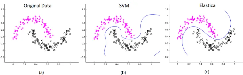
Figure 2: Decision boundaries produced by SVM and EE with common parameters on two moon data.
6. Experimental Results
The proposed two models (TV and EE) are compared with LR, SVM with RBF kernels using the LIBSVM implementation (Chang and Lin, 2011), and Back-Propagation Neural Networks (BPNN) in the Matlab neural network toolbox. Two implementations of our methods are also compared: Gradient Descent method (GD) and Lagged Linear Equation method (LAG). The maximum number of iterations in GD and LAG is empirically setting as 40. Binary classification, multi-class classification, and regression tasks are tested on synthetic and real-world data sets. We collected real data sets from the libsvm website (Chang and Lin, 2011) and the UCI machine learning repository (Asuncion and Newman, 2013). Some attributes have been removed due to missing entries. Some data sets have a huge number of instances, hence we use only 1000 instances in our experiments. All data sets are scaled into [0,1] before training and testing.
6.1 Synthetic Data
We first compare our EE model and SVM for binary classification on two synthetic data sets: the two moon data and one data set made by ourselves. Fig. 2 and Fig. 3 show the decision boundaries produced by SVM and EE with common parameters. We can see that SVM tends to yield curved or even wiggly decision boundaries to pursue low training errors. In contrast, smooth or even straight decision boundaries with low curvature are favored by EE, hence reducing the risk of overfitting.
Figure 3: Decision boundaries produced by SVM and EE with common parameters on our synthetic data.
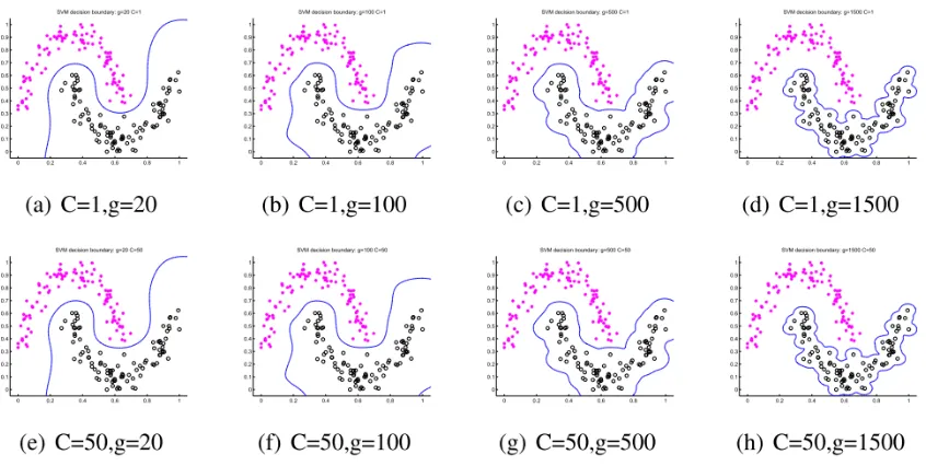
Figure 4: Decision boundaries produced by SVM with different parameter combinations on two moon data.
6.2 Binary Classification
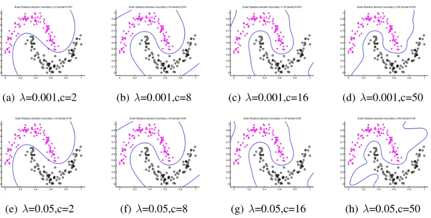
Figure 5: Decision boundaries produced by EE with different parameter combinations on two moon data.
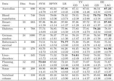
Table 1 gives the average classification accuracies (with standard deviations) for the five methods. The results indicate that BPNN performs the worst, while the LAG version of EE achieves the best accuracies on six data sets. LR and other implementations of TV and EE are comparable with SVM. When comparing EE-LAG and SVM in a pairwise fashion, we can see that EE-LAG achieves improvements over SVM on 10 datasets (though not much statistically significant as the differences on two averaged accuracies is often less than one standard deviation).
6.3 Multi-Class Classification
For multi-class tasks, we collected twelve data sets. For the 256-dimensional USPS data, PCA is used as a preprocessing step to reduce the dimension to 30 and we randomly select 1000 samples for experiments. Same as the settings for binary problems, we use ten runs 5-fold cross-validation to choose the optimal parameters for each method. All methods except for BPNN have two common parameters which are searched from −10 : 10 in logarithm with step 1.
dis-Data Dim Num SVM BPNN LR TV EE GD LAG GD LAG Australian 14 690 85.94 85.34 87.06 87.11 87.01 86.54 87.25
±2.70 ±1.97 ±2.45 ±2.06 ±2.46 ±2.31 ±2.01 Blood 4 748 79.01 79.08 79.32 79.55 79.42 79.73 79.73
transfusion ±3.01 ±3.36 ±3.74 ±2.38 ±2.60 ±2.18 ±2.03 Breast- 10 683 97.36 96.40 97.60 97.36 97.72 97.13 97.83
cancer ±1.59 ±1.14 ±1.27 ±1.28 ±1.43 ±1.37 ±1.29 Diabetes 8 768 77.73 76.85 77.96 77.83 77.81 78.23 78.10
±3.03 ±4.22 ±3.50 ±3.19 ±2.73 ±2.54 ±2.63 German. 24 1000 77.10 76.37 77.10 76.19 77.10 76.50 77.22
number ±1.61 ±1.61 ±1.36 ±1.47 ±1.29 ±1.59 ±1.30 Haberman’s 3 306 74.51 74.52 75.77 75.30 75.28 75.65 75.34 survival ±4.31 ±3.53 ±3.00 ±3.31 ±3.78 ±3.42 ±3.32 Heart 13 270 83.70 81.76 84.26 84.45 84.58 84.78 84.96
±2.72 ±3.16 ±2.22 ±2.82 ±2.73 ±2.69 ±2.79 Liver- 6 345 73.62 71.52 73.20 74.81 73.62 74.32 73.91 disorders ±5.72 ±4.44 ±2.95 ±2.49 ±2.65 ±2.29 ±2.83 Planning 12 182 73.63 67.62 72.22 71.67 71.67 72.22 71.67 relax ±4.41 ±4.93 ±4.46 ±4.93 ±4.08 ±4.25 ±4.79 Sonar 60 208 89.90 88.99 90.88 90.30 90.27 90.07 90.50
±4.41 ±4.79 ±3.83 ±4.47 ±4.72 ±3.27 ±3.37 Vertebral 6 310 85.81 85.16 84.52 84.55 84.75 85.83 85.92
column ±4.26 ±3.12 ±3.90 ±4.14 ±4.37 ±3.38 ±3.68
Table 1: Average accuracies (%) for binary classification with 5-fold cross-validation.
cussions between OVA and OVO. Recently in Varshney and Willsky (2010), an efficient binary encoding strategy was proposed to represent the decision boundary by using only m=dlog2Me functions. Empirically we compared the log2M strategy and the OVA strat-egy for LR, TV and EE, and found that the in most cases the log2M strategy performs slightly better. As the codewords for making decisions are represented as 0-1 bits of length m, the log2M strategy may somehow “favor” those methods with good function approxi-mation ability. In multi-class experiments, thelog2M strategy is used for LR, TV and EE, while LIBSVM runs with the OVO strategy.
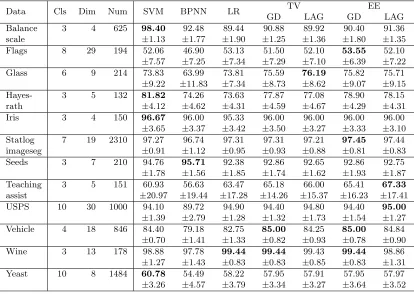
The multi-class results of classification accuracies are shown in Table 2. The accuracy results demonstrate that both SVM and EE-GD offer the best accuracies on four (different) data sets, and both EE-LAG and TV-GD take the first place on two (different) data sets. If we compare SVM and EE-GD in a pairwise fashion by excluding other competing methods, the results show that SVM wins on only five data sets while EE-GD performs better on the other seven data sets. Therefore on multi-class tasks, Table 2 implies that our EE-GD version can offer competitive results, or can perform slightly better than SVM.
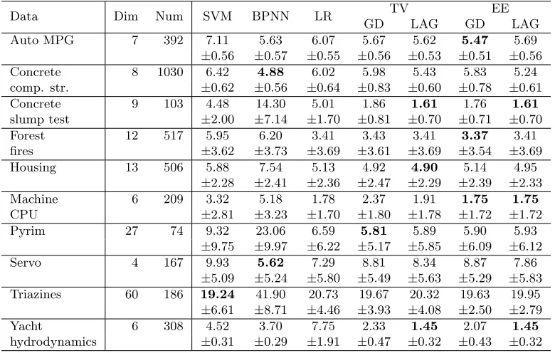
6.4 Regression