On the Convergence Rate of lp-Norm Multiple Kernel Learning

On the Convergence Rate of

ℓ

p

-Norm Multiple Kernel Learning

∗

Marius Kloft† [email protected]

Machine Learning Laboratory Technische Universit¨at Berlin Franklinstr. 28/29

10587 Berlin, Germany

Gilles Blanchard [email protected]

Department of Mathematics University of Potsdam Am Neuen Palais 10 14469 Potsdam, Germany

Editor:S¨oren Sonnenburg, Francis Bach, and Cheng Soog Ong

Abstract

We derive an upper bound on the local Rademacher complexity ofℓp-norm multiple kernel learn-ing, which yields a tighter excess risk bound than global approaches. Previous local approaches analyzed the casep=1 only while our analysis covers all cases 1≤p_≤∞, assuming the different feature mappings corresponding to the different kernels to be uncorrelated. We also show a lower bound that shows that the bound is tight, and derive consequences regarding excess loss, namely fast convergence rates of the orderO(n−1+αα)_{, where}α_{is the minimum eigenvalue decay rate of the}

individual kernels.

Keywords: multiple kernel learning, learning kernels, generalization bounds, local Rademacher complexity

1. Introduction

Propelled by the increasing “industrialization” of modern application domains such as bioinformat-ics or computer vision leading to the accumulation of vast amounts of data, the past decade expe-rienced a rapid professionalization of machine learning methods. Sophisticated machine learning solutions such as the support vector machine can nowadays almost completely be applied out-of-the-box (Bouckaert et al., 2010). Nevertheless, a displeasing stumbling block towards the complete automatization of machine learning remains that of finding the best abstraction orkernel(Sch¨olkopf et al., 1998; M¨uller et al., 2001) for a problem at hand.

In the current state of research, there is little hope that in the near future a machine will be able

to automatically engineer theperfect kernel for a particular problem (Searle, 1980). However, by

restricting to a less general problem, namely to a finite set of base kernels the algorithm can pick

∗. This is a longer version of a short conference paper entitledThe Local Rademacher Complexity ofℓp-Norm MKL, which is appearing in Advances in Neural Information Processing Systems 24 edited by J. Shawe-Taylor and R.S. Zemel and P. Bartlett and F. Pereira and K.Q. Weinberger (2011).

from, one might hope to achieve automatic kernel selection: clearly, cross-validation based model selection (Stone, 1974) can be applied if the number of base kernels is decent. Still, the performance of such an algorithm is limited by the performance of the best kernel in the set.

In the seminal work of Lanckriet et al. (2004) it was shown that it is computationally feasible to simultaneously learn a support vector machineanda linear combination of kernels at the same time, if we require the so-formed kernel combinations to be positive definite and trace-norm normalized.

Though feasible for small sample sizes, the computational burden of this so-calledmultiple kernel

learning(MKL) approach is still high. By further restricting the multi-kernel class to only contain convex combinations of kernels, the efficiency can be considerably improved, so that ten thousands of training points and thousands of kernels can be processed (Sonnenburg et al., 2006).

However, these computational advances come at a price. Empirical evidence has accumulated showing that sparse-MKL optimized kernel combinations rarely help in practice and frequently are

to be outperformed by a regular SVM using an unweighted-sum kernelK=∑mKm(Cortes et al.,

2008; Gehler and Nowozin, 2009), leading for instance to the provocative question “Can learning kernels help performance?” (Cortes, 2009).

A first step towards a model of learning the kernel that is useful in practice was achieved in Kloft et al. (2008), Cortes et al. (2009), Kloft et al. (2009) and Kloft et al. (2011), where anℓq-norm,q≥1,

rather than anℓ1penalty was imposed on the kernel combination coefficients. Theℓq-norm MKL is

an empirical minimization algorithm that operates on the multi-kernel class consisting of functions

f :x_{7→ h}w,φk(x)i with kwk_k ≤D, where φk is the kernel mapping into the reproducing kernel

Hilbert space (RKHS)

H

_kwith kernelkand norm_k._kk, while the kernelkitself ranges over the set of possible kernelsk=∑Mm=1θmkm

kθ_kq≤1,θ≥0 .

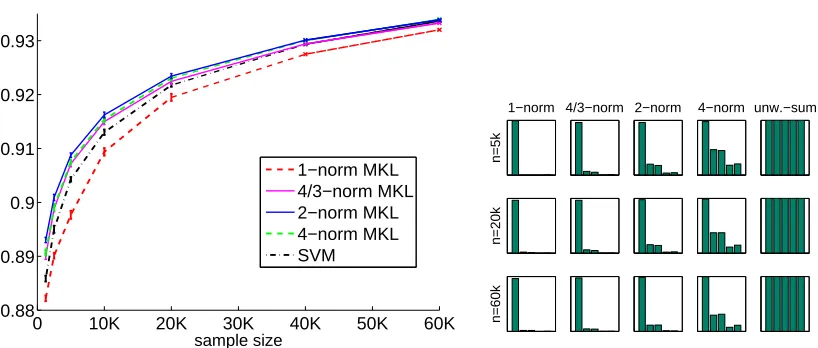
In Figure 1, we reproduce exemplary results taken from Kloft et al. (2009, 2011) (see also references therein for further evidence pointing in the same direction). We first observe that, as expected,ℓq-norm MKL enforces strong sparsity in the coefficientsθmwhenq=1, and no sparsity

at all forq=∞, which corresponds to the SVM with an unweighted-sum kernel, while intermediate

values ofq enforce different degrees of soft sparsity (understood as the steepness of the decrease of the ordered coefficientsθm). Crucially, the performance (as measured by the AUC criterion) is

not monotonic as a function ofq;q=1 (sparse MKL) yields significantly worse performance than

q=∞(regular SVM with sum kernel), but optimal performance is attained for some intermediate

value ofq. This is an empirical strong motivation to theoretically study the performance ofℓq-MKL

beyond the limiting casesq=1 orq=∞.

A conceptual milestone going back to the work of Bach et al. (2004) and Micchelli and Pontil (2005) is that the above multi-kernel class can equivalently be represented as a block-norm regu-larized linear class in the product Hilbert space

H

:=

H

_{1× ··· ×}

H

_M, where

H

_mdenotes the RKHS

associated to kernel km, 1≤m≤M. More precisely, denoting byφm the kernel feature mapping

associated to kernelkm over input space

X

, and φ:x∈

X

7→(φ1(x), . . . ,φM(x))∈

H

, the class of

functions defined above coincides with

Hp,D,M=

fw:x7→ hw,φ(x)i

w= (w(1), . . . ,w(M)),_kw_k2,p≤D , (1)

where there is a one-to-one mapping ofq_∈[1,∞]top_∈[1,2]given by p=_q2q₊₁ (see Appendix A for a derivation). The ℓ2,p-norm is defined here as

w_2,p := _kw(1)_k

k1, . . . ,kw (M)_k

kM_p = ∑Mm=1

w(m)_kp

m

1/p

; for simplicity, we will frequently writew(m)₂=w(m)_k

0 10K 20K 30K 40K 50K 60K 0.88

0.89 0.9 0.91 0.92 0.93

sample size

AUC 1−norm MKL

4/3−norm MKL 2−norm MKL 4−norm MKL SVM

1−norm

n=5k

4/3−norm 2−norm 4−norm unw.−sum

n=20k

n=60k

Figure 1: Splice site detection experiment in Kloft et al. (2009, 2011). LEFT: The Area under ROC curve as a function of the training set size is shown. The regular SVM is equivalent to

q=∞(orp=2). RIGHT: The optimal kernel weightsθmas output byℓq-norm MKL are

shown.

Clearly, the complexity of the class (1) will be greater than one that is based on a single kernel only. However, it is unclear whether the increase is decent or considerably high and—since there is a free parameter p—how this relates to the choice ofp. To this end the main aim of this paper is to analyze the sample complexity of the above hypothesis class (1). An analysis of this model, based on global Rademacher complexities, was developed by Cortes et al. (2010). In the present work,

we base our main analysis on the theory of localRademacher complexities, which allows to derive

improved and more precise rates of convergence.

1.1 Outline of the Contributions

This paper makes the following contributions:

• Upper bounds on the local Rademacher complexity ofℓp-norm MKL are shown, from which

we derive an excess risk bound that achieves a fast convergence rate of the order

O(M1+1+2α p1∗−1

n−1+αα)_{, where}α _{is the minimum eigenvalue decay rate of the individual}

kernels1(previous bounds forℓp-norm MKL only achievedO(M

1

p∗_n−12).

• A lower bound is shown that besides absolute constants matches the upper bounds, showing

that our results are tight.

• The generalization performance ofℓp-norm MKL as guaranteed by the excess risk bound is

studied for varying values of p, shedding light on the appropriateness of a small/large pin various learning scenarios.

Furthermore, we also present a simple proof of a global Rademacher bound similar to the one shown in Cortes et al. (2010). A comparison of the rates obtained with local and global Rademacher analysis, respectively, can be found in Section 6.1.

1.2 Notation

For notational simplicity we will omit feature maps and directly view φ(x) and φm(x) as

ran-dom variablesxandx(m) taking values in the Hilbert space

H

and

H

_m, respectively, wherex=

(x(1)_{, . . . ,x}(M)_{). Correspondingly, the hypothesis class we are interested in reads H}

p,D,M =

fw:

x_{7→ h}w,x_{i k}w_k2,p≤D .IfDorM are clear from the context, we sometimes synonymously

denoteHp=Hp,D=Hp,D,M. We will frequently use the notation (u(m))Mm=1 for the element u=

(u(1), . . . ,u(M))_∈

H

=

H

1×. . .×

H

M.

We denote the kernel matrices corresponding tokandkmbyK andKm, respectively. Note that

we are considering normalized kernel Gram matrices, that is, thei jth entry ofKis 1_nk(xi,xj). We

will also work with covariance operators in Hilbert spaces. In a finite dimensional vector space, the

(uncentered) covariance operator can be defined in usual vector/matrix notation asExx⊤. Since

we are working with potentially infinite-dimensional vector spaces, we will use instead ofxx⊤the tensor notationx_⊗x_∈HS(

H

), which is a Hilbert-Schmidt operator

H

_7→

H

defined as(x_⊗x)u= hx,u_ix. The space HS(

H

) of Hilbert-Schmidt operators on

H

is itself a Hilbert space, and the expectationEx_⊗xis well-defined and belongs to HS(

H

) as soon asEkx_k2 is finite, which will always be assumed (as a matter of fact, we will often assume that_kx_kis bounded a.s.). We denote byJ=Ex_⊗x,Jm=Ex(m)⊗x(m)the uncentered covariance operators corresponding to variables

x,x(m)_{; it holds that tr(J) =Ekxk}2

2and tr(Jm) =E

x(m)2

2.

Finally, for p_∈[1,∞]we use the standard notation p∗ to denote the conjugate of p, that is,

p∗_∈[1,∞]and 1_p+ 1 p∗=1.

2. Global Rademacher Complexities in Multiple Kernel Learning

We first review global Rademacher complexities (GRC) in MKL. Letx1, . . . ,xnbe an i.i.d. sample

drawn fromP. The global Rademacher complexity is defined as

R(Hp) =E sup fw∈Hp

hw,1

n

n

∑

i=1

σixii (2)

where(σi)1≤i≤nis an i.i.d. family (independent of(xi)) of Rademacher variables (random signs).

Its empirical counterpart is denoted by R(Hb p) =

ER(Hp)

x1, . . . ,xn=Eσsupfw∈Hphw,

1 n∑

n

i=1σixii. The interest in the global Rademacher

com-plexity comes from that if known it can be used to bound the generalization error (Koltchinskii, 2001; Bartlett and Mendelson, 2002).

In the recent paper of Cortes et al. (2010) it was shown using a combinatorial argument that the empirical version of the global Rademacher complexity can be bounded as

b

R(Hp)≤D

s

cp∗

2n

tr(Km)

M m=1

p∗

2

,

wherec=23

We will now show a quite short proof of this result, extending it to the whole rangep∈[1,∞], but at the expense of a slightly worse constant, and then present a novel bound on the population version of the GRC. The proof presented here is based on the Khintchine-Kahane inequality (Kahane, 1985) using the constants taken from Lemma 3.3.1 and Proposition 3.4.1 in Kwapi´en and Woyczy´nski (1992).

Lemma 1(Khintchine-Kahane inequality). Let bev1, . . . ,vM∈

H

. Then, for any q≥1, it holds Eσ

_∑

n

i=1

σivi

q

2≤

c

n

∑

i=1

vi

2

2

q

2

,

where c=max(1,q∗₋1). In particular the result holds for c=q∗.

Proposition 2 (Global Rademacher complexity, empirical version). For any p_≥1 the empirical version of global Rademacher complexity of the multi-kernel class Hpcan be bounded as

∀t_≥p: R(Hb p)≤D

s

t∗

n

tr(Km)

M m=1

t∗

2

.

Proof First note that it suffices to prove the result fort=pas trivially_kx_{k2,t ≤ k}x_k2,pholds for all

t_≥pand thereforeR(Hp)≤R(Ht).

We can use a block-structured version of H¨older’s inequality (cf. Lemma 15) and the Khintchine-Kahane (K.-K.) inequality (cf. Lemma 1) to bound the empirical version of the global Rademacher complexity as follows:

b

R(Hp) def.

= Eσ sup

fw∈Hp hw,1

n

n

∑

i=1

σixii

H¨older

≤ DEσ

1_n

n

∑

i=1

σixi

_2,p∗

Jensen

≤ DEσ

M

∑

m=1

1_n

n

∑

i=1

σix(im)

p

∗

2

1

p∗

K.-K.

≤ D

r

p∗ n

M

∑

m=1

₁

n

n

∑

i=1

x(_im)2₂

| {z }

=tr(Km)

p∗

2

1

p∗

=D

s

p∗

n

tr(Km)

M m=1

p∗

2

,

what was to show.

Note that there is a very good reason to state the above bound in terms oft_≥pinstead of solely in terms of p: the Rademacher complexityR(Hb p)is not monotonic in p and thus it is not always

the best choice to taket:= pin the above bound. This can be readily seen, for example, for the

easy case where all kernels have the same trace—in that case the bound translates intoR(Hb p)≤

D

q

t∗Mt2∗ tr(K1)

n . Interestingly, the functionx7→xM

x=2 logM, where log denotes the natural logarithm with respect to the basee. This has interesting consequences: for any p_≤(2 logM)∗_{we can take the boundR(Hb p)≤D}qelog(M)tr(K1)

n , which has

only a mild dependency on the number of kernels; note that in particular we can take this bound for theℓ1-norm classR(Hb 1)for allM>1.

The above proof is very simple. However, computing the population version of the global Rademacher complexity of MKL is somewhat more involved and to the best of our knowledge has not been addressed yet by the literature. To this end, note that from the previous proof we obtain

R(Hp)≤ED

p

p∗_{/n ∑}M m=1 1n∑

n i=1

x(_im)2₂

p∗

2 1

p∗_{. We thus can use Jensen’s inequality to move the}

expectation operator inside the root,

R(Hp)≤D

p

p∗/n

M

∑

m=1 E 1

n

n

∑

i=1

x(_im)2₂

p∗

2

1

p∗

, (3)

but now need a handle on the p₂∗-th moments. To this aim we use the inequalities of Rosenthal

(1970) and Young (e.g., Steele, 2004) to show the following Lemma.

Lemma 3(Rosenthal + Young). Let X1, . . . ,Xnbe independent nonnegative random variables

sat-isfying_∀i:Xi≤B<∞almost surely. Then, denoting Cq= (2qe)q, for any q≥1₂ it holds E

1

n

n

∑

i=1

Xi

q

≤Cq

_B

n

q

+1

n

n

∑

i=1 EXi

q .

The proof is defered to Appendix B. It is now easy to show:

Corollary 4 (Global Rademacher complexity, population version). Assume the kernels are uni-formly bounded, that is,_kk_k∞≤B<∞, almost surely. Then for any p_≥1the population version of global Rademacher complexity of the multi-kernel class Hpcan be bounded as

∀t_≥p: R(Hp,D,M)≤D t∗

r

e n

tr(Jm)

M m=1

t∗

2

+ √

BeDMt1∗t∗

n .

For t_≥2the right-hand term can be discarded and the result also holds for unbounded kernels.

Proof As above in the previous proof it suffices to prove the result fort=p. From (3) we conclude by the previous Lemma

R(Hp)≤D

r

p∗

n

M

∑

m=1

(ep∗)p2∗

_B

n

p∗

2

+E1

n

n

∑

i=1

x(_im)2₂

| {z }

=tr(Jm)

p∗

2 !

1

p∗

≤Dp∗

r_e

n

tr(Jm)M_m=1

p∗

2

+ √

BeDMp1∗_p∗

n ,

where for the last inequality we use the subadditivity of the root function. Note that for p_≥2 it is

p∗/2_≤1 and thus it suffices to employ Jensen’s inequality instead of the previous lemma so that we come along without the last term on the right-hand side.

For example, when the traces of the kernels are bounded, the above bound is essentially determined

by Op∗M

1

p∗

√_n . We can also remark that by settingt= (log(M))∗ we obtain the bound R(H1) =

2.1 Relation to Other Work

As discussed by Cortes et al. (2010), the above results lead to a generalization bound that improves on a previous result based on covering numbers by Srebro and Ben-David (2006). Another recently proposed approach to theoretically study MKL uses the Rademacher chaos complexity (RCC) (Ying and Campbell, 2009). The RCC is actually itself an upper bound on the usual Rademacher com-plexity. In their discussion, Cortes et al. (2010) observe that in the case p=1 (traditional MKL),

the bound of Proposition 2 grows logarithmically in the number of kernelsM, and claim that the

RCC approach would lead to a bound which is multiplicative inM. However, a closer look at the

work of Ying and Campbell (2009) shows that this is not correct; in fact the RCC also leads to a

logarithmic dependence inMwhen p=1. This is because the RCC of a kernel class is the same as

the RCC of its convex hull, and the RCC of the base class containing only theMindividual kernels

is logarithmic inM. This convex hull argument, however, only works for p=1; we are unaware

of any existing work trying to estimate the RCC or comparing it to the above approach in the case

p>1.

3. The Local Rademacher Complexity of Multiple Kernel Learning

We first give a gentle introduction to local Rademacher complexities in general and then present the main result of this paper: a lower and an upper bound on the local Rademacher complexity of

ℓp-norm multiple kernel learning.

3.1 Local Rademacher Complexities in a Nutshell

Letx1, . . . ,xnbe an i.i.d. sample drawn fromP; denote byEthe expectation operator corresponding

toP; let

F

be a class of functions mapping xi to R. Then the local Rademacher complexity is

defined as

Rr(

F

) =E sup f∈F:P f2_≤r

1

n

n

∑

i=1

σif(xi), (4)

whereP f2:=E(f(x))2_{. In a nutshell, when comparing the global and local Rademacher}

complex-ities, that is, (2) and (4), we observe that the local one involves the additional constraintP f2_≤r

on the (uncentered) “variance” of functions. It allows us to sort the functions according to their variances and discard the ones with suboptimal high variance. We can do so by, instead of McDi-armid’s inequality, using more powerful concentration inequalities such as Talagrand’s inequality (Talagrand, 1995). Roughly speaking, the local Rademacher complexity allows us to consider the problem at various scales simultaneously, leading to refined bounds. We will discuss this argument in more detail now. Our presentation is based on Koltchinskii (2006).

First, note that the classical (global) Rademacher theory of Bartlett and Mendelson (2002) and Koltchinskii (2001) gives an excess risk bound of the following form:_∃C>0 so that with probabil-ity larger then 1₋exp(₋t)it holds

Pfˆ−P f∗≤C

R(

F

) +

r

t n

=:δ, (5)

where ˆf:=argmin_f∈F 1n∑ n

i=1f(xi), f∗:=argminf∈FP f, andP f:=Ef(x). We denote the bound’s

F

_δ:=_{f ∈

F

:_|P f−P f∗| ≤δ_}, we have by (5) that ˆf ∈

F

_δ (and trivially f∗∈

F

_δ). This is re-markable and of significance because we can now state: with probability larger than 1₋exp(₋2t)

it holds

Pfˆ₋P f∗_≤C

R(

F

_δ) +

r

t n

. (6)

The striking fact about the above inequality is that it depends on the complexity of the restricted class—no longer on the one of the original class; usually the complexity of the restricted class will be smaller than the one of the original class. Moreover, we can again denote the right-hand side of (6) byδnew_{and repeat the argumentation. This way, we can step by step decrease the bound’s value.}

If the bound (seen as a function inδ) defines a contraction, the limit of this iterative procedure is given by the fixed point of the bound.

This method has a serious limitation: although we can step by step decrease the Rademacher complexity occurring in the bound, the termpt/nstays as it is and thus will hinder us from attaining

a rate faster than O(p1/n). It would be desirable to have the term shrinking when passing to

a smaller class

F

_δ. Can we replace the undesirable term by a more favorable one? And what

properties would such a term need to have?

One of the basic foundations of learning theory are concentration inequalities (e.g., Bousquet et al., 2004). Even the most modern proof technique such as the fixed-point argument presented above can fail if it is built upon an insufficiently precise concentration inequality. As mentioned

above, the stumbling block is the presence of the term pt/n in the bound (5). The latter is a

byproduct from the application of McDiarmid’s inequality (McDiarmid, 1989)—a uniform version of H¨offding’s inequality—,which is used in Bartlett and Mendelson (2002) and Koltchinskii (2001) to relate the global Rademacher complexity with the excess risk.

The core idea now is that we can, instead of McDiarmid’s inequality, use Talagrand’s inequality (Talagrand, 1995), which is a uniform version of Bernstein’s inequality. This gives

Pfˆ₋P f∗_≤C

R(

F

) +σ(

F

)

r

t n+

t n

=:δ. (7)

Herebyσ2₍

_F

_):=sup

f∈FEf2is a bound on the (uncentered) “variance” of the functions considered. Now, denoting the right-hand side of (7) byδ, we obtain the following bound for the restricted class:

∃C>0 so that with probability larger then 1₋exp(₋2t)it holds

Pfˆ₋P f∗_≤C

R(

F

_δ) +σ(

F

_δ)

r

t n+

t n

. (8)

As above, we denote the right-hand side of (8) byδnew_{and repeat the argumentation. In general, we}

can expect the varianceσ2₍

_F

δ)to decrease step by step and if, seen as a function of δ, the bound defines a contraction, the limit is given by the fixed point of the bound.

It turns out that by this technique we can obtain fast convergence rates of the excess risk in the

number of training examplesn, which would be impossible by using global techniques such as the

3.2 The Local Rademacher Complexity of MKL

In the context ofℓp-norm multiple kernel learning, we consider the hypothesis classHp as defined

in (1). Thus, given an i.i.d. samplex1, . . . ,xn drawn fromP, the local Rademacher complexity is

given byRr(Hp) =Esupfw∈Hp:P fw2≤rhw,

1 n∑

n

i=1σixii, whereP fw2 :=E(fw(x))2.

We will need the following assumption for the case 1_≤p_≤2:

Assumption (A) (low-correlation). There exists a cδ∈(0,1]such that, for any m6=m′andwm∈

H

_m,wm′ ∈

H

_m′, the Hilbert-space-valued variablesx(1), . . . ,x(M)satisfy

cδ

M

∑

m=1

EDwm,x(m)

E2

≤E M

∑

m=1

D

wm,x(m)E2.

Since

H

m,

H

m′ are RKHSs with kernels km,km′, if we go back to the input random variable in the original space X _∈

X

, the above property means that for any fixedt,t′ _∈

X

, the variables

km(X,t)andkm′(X,t′) have alow correlation. In the most extreme case,c_δ=1, the variables are

completely uncorrelated. This is the case, for example, if the original input space

X

is RM, the

original input variableX _∈

X

has independent coordinates, and the kernelsk1, . . . ,kM each act on

a different coordinate. Such a setting was considered in particular by Raskutti et al. (2010) in the setting ofℓ1-penalized MKL. We discuss this assumption in more detail in Section 6.3.

Note that, as self-adjoint, positive Hilbert-Schmidt operators, covariance operators enjoy dis-crete eigenvalue-eigenvector decompositions J =Ex_⊗x=∑∞j=1λjuj⊗uj and Jm =Ex(m)⊗

x(m)_=∑∞

j=1λ

(m)

j u

(m)

j ⊗u

(m)

j , where(uj)j≥1and(u(jm))j≥1form orthonormal bases of

H

and

H

m,

respectively.

We are now equipped to state our main results:

Theorem 5 (Local Rademacher complexity, p∈[1,2]). Assume that the kernels are uniformly bounded (_kk_k∞≤B<∞) and that Assumption(A)holds. The local Rademacher complexity of the multi-kernel class Hpcan be bounded for any1≤p≤2as

∀t_∈[p,2]: Rr(Hp)≤

v u u t16

n

∞

∑

j=1

minrM1−t2∗,ceD2t∗2λ(m)

j

M

m=1

t∗

2

+ √

BeDMt1∗t∗

n .

Theorem 6(Local Rademacher complexity,p_≥2). The local Rademacher complexity of the multi-kernel class Hpcan be bounded for any p≥2as

Rr(Hp)≤

s

2

n ∞

∑

j=1

min(r,D2_Mp2∗−1λ

j).

Remark 7. Note that for the case p=1, by using t= (log(M))∗ _{in Theorem 5, we obtain the bound}

Rr(H1)≤

v u u t16

n

∞

∑

j=1

min

rM,e3_D2_(logM)2_λ(m) j

M

m=1

∞ +

√

Be32Dlog(M)

n ,

Remark 8. The result of Theorem 6 for p≥2 can be proved using considerably simpler tech-niques and without imposing assumptions on boundedness nor on uncorrelation of the kernels. If in addition the variables (x(m)) are centered and uncorrelated, then the spectra are related as follows : spec(J) =SM

m=1spec(Jm); that is, {λi,i≥1}=SMm=1

n

λ(_im),i≥1

o

. Then one can

write equivalently the bound of Theorem 6 as Rr(Hp)≤

q

2 n∑

M

m=1∑∞j=1min(r,D2M

2

p∗−1_λ(m)

j ) =

r

2 n

∑∞j=1min(r,D2M

2

p∗−1λ(m)

j )

M

m=1

1. However, the main intended focus of this paper is on the

more challenging case1_≤p_≤2which is usually studied in multiple kernel learning and relevant in practice.

Remark 9. It is interesting to compare the above bounds for the special case p=2with the ones of Bartlett et al. (2005). The main term of the bound of Theorem 6 (taking t =p=2) is then essentially determined by Oq1_n∑Mm=1∑∞j=1min r,λ

(m)

j

. If the variables(x(m))are centered and uncorrelated, by the relation between the spectra stated in Remark 8, this is equivalently of order Oq1_n∑∞j=1min r,λj

, which is also what we obtain through Theorem 6, and coincides with the rate shown in Bartlett et al. (2005).

Proof of Theorem 5 The proof is based on first relating the complexity of the class Hp with its

centered counterpart, that is, where all functions fw∈Hpare centered around their expected value.

Then we compute the complexity of the centered class by decomposing the complexity into blocks, applying the no-correlation assumption, and using the inequalities of H¨older and Rosenthal. Then we relate it back to the original class, which we in the final step relate to a bound involving the truncation of the particular spectra of the kernels. Note that it suffices to prove the result fort=p

as triviallyR(Hp)≤R(Ht)for allp≤t.

STEP1: RELATING THE ORIGINAL CLASS WITH THE CENTERED CLASS. In order to exploit the no-correlation assumption, we will work in large parts of the proof with the centered class

˜

Hp =

_˜

fw

_kw_k2,p≤D , wherein ˜fw:x7→ hw,x˜i, and ˜x:=x−Ex. We start the proof by noting that ˜fw(x) = fw(x)− hw,Exi= fw(x)−Ehw,xi = fw(x)−Efw(x), so that, by the bias-variance decomposition, it holds that

P f_w2 =Efw(x)2=E(fw(x)−Efw(x))2+ (Efw(x))2=Pf˜w2 + P fw

2

. (9)

Furthermore we note that by Jensen’s inequality

_Ex_2,p∗ =

M

∑

m=1

_Ex(m)₂p∗

1

p∗ =

M

∑

m=1

Ex(m),Ex(m)

p∗

2

1

p∗

Jensen

≤

M

∑

m=1

Ex(m),x(m)

p∗

2

1

p∗ =

s

tr(Jm)

M

m=1

p∗

2

so that we can express the complexity of the centered class in terms of the uncentered one as follows:

Rr(Hp) =E sup fw∈Hp,

P f2

w≤r

w,1

n

n

∑

i=1

σixi

≤E sup

fw∈Hp,

P fw2≤r

w,1

n

n

∑

i=1

σix˜i +E sup fw∈Hp,

P fw2≤r

w,1

n

n

∑

i=1

σiEx

Concerning the first term of the above upper bound, using (9) we havePf˜_w2 _≤P f_w2 , and thus

E sup

fw∈Hp,

P fw2≤r

w,1

n

n

∑

i=1

σix˜i≤E sup fw∈Hp,

Pf˜w2≤r

w,1

n

n

∑

i=1

σix˜i=Rr(H˜p).

Now to bound the second term, we write

E sup

fw∈Hp,

P fw2≤r

w,1

n

n

∑

i=1

σiEx=E

1

n

n

∑

i=1

σi

fwsup∈Hp,

P fw2≤r

hw,Ex_i

≤ sup

fw∈Hp,

P fw2≤r

w,Ex

 _E 1

n

n

∑

i=1

σi

!2



1 2

=√n sup

fw∈Hp,

P f2

w≤r

hw,Ex_i.

Now observe finally that we have

hw,Ex_iH¨older_{≤ k}w_k2,pkEx_k2,p∗

(10)

≤ kw_k2,p

r

tr(Jm)M_m=1

p∗

2

as well as

hw,Ex_i=Efw(x)≤

q

P f2

w.

We finally obtain, putting together the steps above,

Rr(Hp)≤Rr(H˜p) +n−

1 2min

_√

r,D

r tr(Jm)

M m=1

p∗

2

(11)

This shows that we at the expense of the additional summand on the right hand side we can work with the centered class instead of the uncentered one.

STEP 2: BOUNDING THE COMPLEXITY OF THE CENTERED CLASS. Since the (centered) covariance operatorEx˜(m)_⊗x˜(m)is also a self-adjoint Hilbert-Schmidt operator on

H

_m, there exists an eigendecomposition

Ex˜(m)_⊗x˜(m)= ∞

∑

j=1

˜

wherein(u˜(_jm))j≥1 is an orthogonal basis of

H

m. Furthermore, the no-correlation assumption(A)

entailsEx˜(l)_⊗x˜(m)=0for alll₆=m. As a consequence,

Pf˜_w2 = E(fw(x˜))2 = E

M

∑

m=1

wm,x˜(m) 2

=

M

∑

l,m=1

D

wl, Ex˜(l)⊗x˜(m)

wm

E

(A) ≥ cδ

M

∑

m=1

D

wm, Ex˜(m)⊗x˜(m)wm

E

=

M

∑

m=1

∞

∑

j=1

˜

λ(_jm)Dwm,u˜(jm)

E2

(13)

and, for all jandm,

ED1

n

n

∑

i=1

σix˜( m)

i ,u˜

(m)

j

E2

= E1

n2 n

∑

i,l=1

σiσl

D

˜

x_i(m),u˜(_jm)EDx˜_l(m),u˜(_jm)Eσ=i.i.d.E1

n2 n

∑

i=1

D

˜

x(_im),u˜(_jm)E2

= 1

n

D

˜ u(_jm),1

n

n

∑

i=1

Ex˜(_im)_⊗x˜(_im)

| {z }

=Ex˜(m)_⊗x˜(m)

˜ u(_jm)E=

˜

λ(_jm)

n . (14)

Now, let h1, . . . ,hM be arbitrary nonnegative integers. We can express the local Rademacher

complexity in terms of the eigendecomposition (12) as follows

Rr(H˜p) = E sup

fw∈H˜p:Pf˜w2≤r

D

w,1

n

n

∑

i=1

σix˜i

E

= E sup

fw∈H˜p:Pf˜w2≤r

D

w(m)M_m=1, 1

n

n

∑

i=1

σix˜( m)

i

M m=1

E

= E sup

fw∈H˜p:Pf˜w2≤r

w,

∞

∑

j=1

h1_n

n

∑

i=1

σix˜( m)

i ,u˜

(m)

j iu˜

(m)

j

M

m=1

(⋆)

= _E sup

Pf˜2

w≤r

D hm

∑

j=1

q

˜

λ(_jm)_hw(m),u˜(_jm)_iu˜(_jm)M

m=1,

hm

∑

j=1

q

˜

λ(_jm)−

1

h1 n

n

∑

i=1

σix˜(im),u˜

(m)

j iu˜

(m)

j

M

m=1

E

+ _E sup

fw∈H˜p

w,

∞

∑

j=hm+1 h1

n

n

∑

i=1

σix˜(im),u˜

(m)

j iu˜

(m)

j

M

m=1

C.-S., Jensen

≤ sup

Pf˜2

w≤r

" _M

∑

m=1 hm

∑

j=1

˜

λ(_jm)_hw(m),u˜(_jm)_i2

!1 2

×

M

∑

m=1 hm

∑

j=1

˜

λ(_jm)−1E1

n

n

∑

i=1

σix˜(im),u˜

(m)

j

2

!1 2#

+E sup

fw∈H˜p

w,

∞

∑

j=hm+1 h1_n

n

∑

i=1

σix˜(im),u˜

(m)

j iu˜

(m)

j

M

m=1

where for(⋆)we use the linearity of the scalar product, so that (13) and (14) yield

Rr(H˜p)

(13), (14)

≤

s

rc−_δ1∑Mm=1hm

n +E_fsup

w∈H˜p

w,

∞

∑

j=hm+1 h1_n

n

∑

i=1

σix˜( m)

i ,u˜

(m)

j iu˜

(m)

j

M

m=1

H¨older

≤

s

rc−_δ1∑Mm=1hm

n +DE

∞

∑

j=hm+1 h1_n

n

∑

i=1

σix˜( m)

i ,u˜

(m)

j iu˜

(m)

j

M

m=1

₂

,p∗

.

STEP 3: KHINTCHINE-KAHANE’S AND ROSENTHAL’S INEQUALITIES. We can now use the Khintchine-Kahane (K.-K.) inequality (see Lemma 1 in Appendix B) to further bound the right term in the above expression as follows

E ∞

∑

j=hm+1 h1_n

n

∑

i=1

σix˜(_im),u˜(_jm)iu˜(_jm)

M

m=1

_2,p∗

Jensen

≤ E

M

∑

m=1 Eσ ∞

∑

j=hm+1 h1_n

n

∑

i=1

σix˜(im),u˜

(m)

j iu˜

(m)

j p∗ Hm 1 p∗ K.-K. ≤ r p∗ n E M

∑

m=1

∞

∑

j=hm+1

1

n

n

∑

i=1

hx˜(_im),u˜(_jm)_i2

p∗ 2 1 p∗ Jensen ≤ r p∗ n M

∑

m=1 E

∞

∑

j=hm+1

1

n

n

∑

i=1

hx˜(_im),u˜(_jm)_i2

p∗

2

1

p∗

,

Note that for p_≥2 it holds that p∗/2_≤1, and thus it suffices to employ Jensen’s inequality once again in order to move the expectation operator inside the inner term. In the general case we need a

handle on the p₂∗-th moments and to this end employ Lemma 3 (Rosenthal + Young), which yields

M

∑

m=1 E

∞

∑

j=hm+1

1

n

n

∑

i=1

hx˜(_im),u˜(_jm)_i2

p∗ 2 1 p∗ R+Y ≤ M

∑

m=1

(ep∗)p2∗

_B n p∗ 2 + ∞

∑

j=hm+1

1

n

n

∑

i=1

Ehx˜(_im),u˜(_jm)_i2

| {z }

=λ˜(jm)

p∗

2 !

1 p∗ (∗) ≤ v u u

t_ep∗ BM

2

p∗

n +

M

∑

m=1

∞

∑

j=hm+1

˜

λ(_jm) p∗

2

2

p∗!

=

v u u

tep∗ BM

2 p∗ n + ∞

∑

j=hm+1

˜

λ(_jm)

M

m=1

p∗ 2 ! ≤ v u u

tep∗ BM

2 p∗ n + ∞

∑

j=hm+1 λ(_jm)

M

m=1

where for(_∗)we used the subadditivity of p√∗_{·and in the last step we applied the}

Lidskii-Mirsky-Wielandt theorem which gives_∀j,m: ˜λ(_jm)_≤λ(_jm). Thus by the subadditivity of the root function

Rr(H˜p) ≤

s

rc−_δ1∑Mm=1hm

n +D

v u u tep∗2

n

BMp2∗

n + ∞

∑

j=hm+1 λ(_jm)

M

m=1

p∗ 2 ! = s

rc−_δ1∑Mm=1hm

n +

v u u tep∗2D2

n ∞

∑

j=hm+1 λ(_jm)

M

m=1

p∗ 2 + √

BeDMp1∗_p∗

n . (15)

STEP 4: BOUNDING THE COMPLEXITY OF THE ORIGINAL CLASS. Now note that for all

nonnegative integershmwe either have

n−12min

q

rc−_δ1,D

r tr(Jm)

M m=1

p∗ 2 ≤ v u u tep∗2D2

n ∞

∑

j=hm+1 λ(_jm)

M

m=1

p∗ 2

(in case allhmare zero) or it holds

n−21min

q

rc−_δ1,D

r tr(Jm)

M m=1

p∗ 2 ≤ s

rc−_δ1∑Mm=1hm

n

(in case that at least onehmis nonzero) so that in any case we get

n−12min

q

rc−_δ1,D

r tr(Jm)

M m=1

p∗ 2 ≤ s

rc−_δ1∑M_m=1hm

n +

v u u tep∗2D2

n ∞

∑

j=hm+1 λ(_jm)

M

m=1

p∗ 2 . (16)

Thus the following preliminary bound follows from (11) by (15) and (16):

Rr(Hp)≤

s

4rc−_δ1∑Mm=1hm

n +

v u u

t4ep∗2D2

n ∞

∑

j=hm+1 λ(_jm)

M

m=1

p∗ 2 + √

BeDMp1∗_p∗

n , (17)

for all nonnegative integershm≥0. We could stop here as the above bound is already the one that

will be used in the subsequent section for the computation of the excess loss bounds. However, we can work a little more on the form of the bound to gain more insight on its properties—we will show that it is related to the truncation of the spectra at the scaler.

STEP5: RELATING THE BOUND TO THE TRUNCATION OF THE SPECTRA OF THE KERNELS. To this end, notice that for all nonnegative real numbersA1,A2and anya1,a2∈Rm+it holds for all

q_≥1

p

A1+

p

A2 ≤

p

2(A1+A2) (18)

ka1kq+ka2kq ≤ 2 1₋1

q_ka

(the first statement follows from the concavity of the square root function and the second one is proved in appendix B; see Lemma 17) and thus

Rr(Hp)

(18)

≤

v u u t8 rc

−1

δ ∑

M m=1hm

n +

ep∗2D2

n ∞

∑

j=hm+1 λ(_jm)

M

m=1

p∗ 2 ! + √

BeDMp1∗_p∗ n

ℓ1-to-ℓp∗

2 ≤ v u u t8 n rc −1 δ M

1₋2

p∗ hm M

m=1

p∗

2

+ep∗2D2

∞

∑

j=hm+1 λ(_jm)

M

m=1

p∗ 2 ! + √

BeDMp1∗_p∗ n (19) ≤ v u u t16 n

rc−_δ1M1−p2∗_h

m+ep∗2D2

∞

∑

j=hm+1 λ(_jm)

M

m=1

p∗ 2 + √

BeDMp1∗_p∗

n ,

where to obtain the second inequality we applied that for all non-negativea_∈RMand 0<q<p_≤∞

it holds2

(ℓq-to-ℓpconversion) kakq=h1,a q

i1q

H¨older

≤ k1_k(p/q)∗kaqk_p/q

1/q

=M1q−1p_kak

p. (20)

Since the above holds for all nonnegative integershm, it follows

Rr(Hp) ≤

v u u t16 n min

hm≥0

rc−_δ1M1−p2∗_h

m+ep∗2D2

∞

∑

j=hm+1 λ(_jm)

M

m=1

p∗ 2 + √

BeDMp1∗_p∗ n = v u u t16 n ∞

∑

j=1

minrc−_δ1M1−p2∗_,ep∗2_D2_λ(m)

j

M

m=1

p∗ 2 + √

BeDMp1∗_p∗

n ,

which completes the proof of the theorem.

Proof of Remark 7 To see that Remark 7 holds notice thatR(H1)≤R(Hp)for allp≥1 and thus

by choosingp= (log(M))∗_{the above bound implies}

Rr(H1) ≤

v u u t16 n ∞

∑

j=1

minrc−_δ1M1−p2∗,_ep∗2_D2λ(m)

j

M

m=1

p∗ 2 + √

BeDMp1∗_p∗ n

ℓp∗

2

−to−ℓ∞

≤ v u u t16 n ∞

∑

j=1

minrc−_δ1M,ep∗2Mp2∗_D2_λ(m)

j

M

m=1

∞ + √

BeDMp1∗_p∗ n = v u u t16 n ∞

∑

j=1

minrc−_δ1M,e3_D2_(logM)2_λ(m) j

M

m=1

∞ + √

Be32D(logM)

n ,

which completes the proof.

2. We denote byaqthe vector with entriesaq

Proof of Theorem 6.

The eigendecompositionEx_⊗x=∑∞j=1λjuj⊗uj yields

P f_w2 =E(fw(x))2=Ehw,xi2=w,(Ex⊗x)w= ∞

∑

j=1

λj

w,uj

2

, (21)

and, for all j

ED1

n

n

∑

i=1

σixi,uj

E2

= E1

n2 n

∑

i,l=1

σiσl

xi,uj

xl,uj

σi.i.d.

= E1

n2 n

∑

i=1

xi,uj

2

= 1

n

D

uj,

₁

n

n

∑

i=1

Exi⊗xi

| {z }

=Ex_⊗x

uj

E

=λj

n . (22)

Therefore, we can use, for any nonnegative integerh, the Cauchy-Schwarz inequality and a

block-structured version of H¨older’s inequality (see Lemma 15) to bound the local Rademacher complexity as follows:

Rr(Hp) = E sup

fw∈Hp:P fw2≤r

w,1

n

n

∑

i=1

σixi

= E sup

fw∈Hp:P fw2≤r

h

∑

j=1

q

λjhw,ujiuj, h

∑

j=1

q

λj −1

h1_n

n

∑

i=1

σixi,ujiuj

+ w,

∞

∑

j=h+1

h1_n

n

∑

i=1

σixi,ujiuj

C.-S., (21),(22)

≤

r

rh

n +Efwsup∈Hp

w,

∞

∑

j=h+1

h1 n

n

∑

i=1

σixi,ujiuj

H¨older

≤

r

rh n +DE

∞

∑

j=h+1

h1_n

n

∑

i=1

σixi,ujiuj

2,p∗

ℓp∗

2 −

to−ℓ2

≤

r

rh n +DM

1

p∗−

1 2_E ∞

∑

j=h+1

h1 n

n

∑

i=1

σixi,ujiuj

_H Jensen ≤ r rh n +DM

1

p∗−

1 2

∞

∑

j=h+1 Eh1_n

n

∑

i=1

σixi,uji2

| {z }

(22)

≤λj n 1 2 ≤ r rh n + v u u tD2M

2

p∗−1 n

∞

∑

j=h+1

λj.

Since the above holds for allh, the result now follows from√A+√B_≤p2(A+B)for all nonneg-ative real numbersA,B(which holds by the concavity of the square root function):

Rr(Hp)≤

s

2

n0min≤h≤n

rh+D2_Mp2∗−1 ∞

∑

j=h+1

λj = s 2 n ∞

∑

j=1

min(r,D2_Mp2∗−1_λ

4. Lower Bound

In this subsection we investigate the tightness of our bound on the local Rademacher complexity of

Hp. To derive a lower bound we consider the particular case where variablesx(1), . . . ,x(M)are i.i.d.

For example, this happens if the original input space

X

isRM, the original input variableX_∈

X

has i.i.d. coordinates, and the kernelsk1, . . . ,kMare identical and each act on a different coordinate of

X.

Lemma 10. Assume that the variables x(1), . . . ,x(M) are centered and identically independently distributed. Then, the following lower bound holds for the local Rademacher complexity of Hpfor

any p_≥1:

Rr(Hp,D,M) ≥ RrM(H1,DM1/p∗_,1).

Proof First note that since thex(i)are centered and uncorrelated, that

P f_w2 =

M

∑

m=1

wm,x(m)

2

=

M

∑

m=1

wm,x(m)

2 .

Now it follows

Rr(Hp,D,M) = E sup

w: P fw2 ≤r

kwk

2,p≤D

w,1

n

n

∑

i=1

σixi

= E sup

w:∑Mm=1

w(m),x(m)2≤r

kwk_2,p≤D

w,1

n

n

∑

i=1

σixi

≥ E sup

w:

∀m:w(m),x(m)2≤r/M

w(m)

_2,p≤D

w(1)

=···=

w(M)

w,1

n

n

∑

i=1

σixi

= E sup

w:∀m:

w(m),x(m)2≤r/M

∀m:

w(m)

₂≤DM−1p

M

∑

m=1

w(m),1

n

n

∑

i=1

σix(im)

=

M

∑

m=1

E sup

w(m)_:

w(m)_,x(m)2

≤r/M

w(m)

2≤DM

−1

p

w(m),1

n

n

∑

i=1

σix(im)

so that we can use the i.i.d. assumption onx(m)_{to equivalently rewrite the last term as follows:}

Rr(Hp,D,M)

x(m)_i.i.d.

≥ E sup

w(1)_:

w(1)_,x(1)2

≤r/M

w(1)

2≤DM

−1p

Mw(1),1

n

n

∑

i=1

σix(i1)

= _E sup

w(1)_:

Mw(1),x(1)2≤rM

Mw(1)

2≤DM 1

p∗

Mw(1),1

n

n

∑

i=1

σix(i1)

= E sup

w(1)_:

w(1),x(1)2≤rM

w(1)

2≤DM 1

p∗

w(1),1

n

n

∑

i=1

σix(i1)

= RrM(H1,DM1/p∗_,1)

In Mendelson (2003) it was shown that there is an absolute constantcso that ifλ(1)_≥1

n then for all

r≥1

n it holdsRr(H1,1,1)≥

q

c n∑

∞

j=1min(r,λ

(1)

j ). Closer inspection of the proof reveals that more

generally it holdsRr(H1,D,1)≥

q

c n∑

∞

j=1min(r,D2λ

(1)

j )ifλ

(m)

1 ≥nD12 so that we can use that result together with the previous lemma to obtain:

Theorem 11(Lower bound). Assume that the kernels are centered and identically independently distributed. Then, the following lower bound holds for the local Rademacher complexity of Hp.

There is an absolute constant c such that ifλ(1)_≥ 1

nD2 then for all r≥1_n and p≥1,

Rr(Hp,D,M) ≥

s

c n

∞

∑

j=1

min(rM,D2_M2/p∗_λ(1)

j ). (23)

We would like to compare the above lower bound with the upper bound of Theorem 5. To this end note that for centered identical independent kernels the upper bound reads

Rr(Hp)≤

s

16

n ∞

∑

j=1

minrM,ceD2_p∗2_Mp2∗_λ(1)

j

+ √

BeDMp1∗_p∗

n ,

which is of the order O

q

∑∞j=1min rM,D2M

2

p∗_λ(1)

j

and, disregarding the quickly converging term on the right hand side and absolute constants, again matches the upper bounds of the previous section. A similar comparison can be performed for the upper bound of Theorem 6: by Remark 8 the bound reads

Rr(Hp)≤

s 2 n ∞

∑

j=1

min(r,D2_Mp2∗−1_λ(m)

j )

M

m=1

₁,

which for i.i.d. kernels becomes

q

2/n∑∞j=1min rM,D2M

2

p∗λ(1)

j

5. Excess Risk Bounds

In this section we show an application of our results to prediction problems, such as classification or regression. To this aim, in addition to the data x1, . . . ,xn introduced earlier in this paper, let

also a label sequence y1, . . . ,yn⊂[−1,1]be given that is i.i.d. generated from a probability

dis-tribution. The goal in statistical learning is to find a hypothesis f from a pregiven class

F

that

minimizes the expected lossEl(f(x),y), wherel:R27→[₋1,1]is a predefined loss function that encodes the objective of the given learning/prediction task at hand. For example, the hinge loss

l(t,y) =max(0,1₋yt) and the squared lossl(t,y) = (t₋y)2 _{are frequently used in classification}

and regression problems, respectively.

Since the distribution generating the example/label pairs is unknown, the optimal decision func-tion

f∗:=argmin

f∈F E

l(f(x),y)

can not be computed directly and a frequently used method consists of instead minimizing the

empiricalloss,

ˆ

f :=argmin

f∈F 1

n

n

∑

i=1

l(f(xi),yi).

In order to evaluate the performance of this so-calledempirical risk minimization(ERM) algorithm

we study the excess loss,

P(lfˆ−lf∗) := El(fˆ(x),y)−El(f∗(x),y).

In Bartlett et al. (2005) and Koltchinskii (2006) it was shown that the rate of convergence of the excess risk is basically determined by the fixed point of the local Rademacher complexity. For example, the following result is a slight modification of Corollary 5.3 in Bartlett et al. (2005) that is well-tailored to the class studied in this paper.3

Lemma 12. Let

F

be an absolute convex class ranging in the interval[a,b]and let l be a Lipschitz continuous loss with constant L. Assume there is a positive constant F such that

∀f_∈

F

: P(f₋f∗)2_{≤F P(l}

f−lf∗). (24)

Then, denoting by r∗the fixed point of

2FL R r

4L2(

F

)

for all x>0with probability at least1₋e−x the excess loss can be bounded as

P(l_fˆ−lf∗)≤7r

∗

F +

(11L(b₋a) +27F)x

n .

Note that condition (24) on the loss function is fulfilled, for example, when the kernel is uni-formly bounded and the loss function is strongly convex and Lipschitz continuous on the domain considered (Bartlett et al., 2006). This includes, for example, the squared loss as defined above, the

logistic lossl(t,y) =ln(1+exp(₋yt)), and the exponential lossl(t,y) =exp(₋yt). The case of the hinge loss (see definition above) is more delicate, since it is not a strongly convex loss function. In general, the hinge loss does not satisfy (24) on an arbitrary convex class

F

; for this reason, there is no direct, general “fast rate” excess loss analogue to the popular margin-radius bounds obtained through global Rademacher analysis. Nevertheless, local Rademacher complexity analysis can still be put to good use for algorithms based on the hinge loss. In fact, the hinge loss satisfies, under an additional ”noise exponent condition” assumption, a restricted version of (24), namely, when f∗is taken equal to the Bayes classifier. This can be used to study theoretically the behavior of penal-ized ERM methods such as the support vector machine, and more precisely to obtain oracle-type inequalities (this roughly means that the penalized ERM can be shown to pick a correct trade-off of bias and estimation error, leading to fast convergence rates). In this sense, the local Rademacher complexity bound we have presented here can in principle be plugged in into the SVM analysis of Blanchard et al. (2008), directly replacing the local Rademacher analysis for a single kernel studied there under setting (S1); see also Steinwart and Christmann (2008, Chapter 8) for a comparable analysis. This more elaborate analysis does, however, not fall directly into the scope of the com-parably simpler result of Lemma 12, which considers simple ERM over a fixed model, so that we refer the reader to the references cited above for more details.

Lemma 12 shows that in order to obtain an excess risk bound on the multi-kernel class Hp it

suffices to compute the fixed point of our bound on the local Rademacher complexity presented in Section 3. To this end we show:

Lemma 13. Assume thatkkk∞≤B almost surely and assumption (A) holds; let p∈[1,2]. For the fixed point r∗of the local Rademacher complexity 2FLR r

4L2(Hp) it holds

r∗_≤ min

0_≤hm≤∞

4c−_δ1F2∑Mm=1hm

n +8FL

v u u tep∗2D2

n

∞

∑

j=hm+1 λ(_jm)

M

m=1

p∗

2

+4

√

BeDFLMp1∗_p∗

n .

Proof For this proof we make use of the bound (17) on the local Rademacher complexity. Defining

a=4c

−1

δ F2∑Mm=1hm

n and b=4FL

v u u tep∗2D2

n

∞

∑

j=hm+1 λ(_jm)

M

m=1

p∗

2

+2

√

BeDFLMp1∗_p∗

n ,

in order to find a fixed point of (17) we need to solve forr=√ar+b, which is equivalent to solving

r2₋(a+2b)r+b2=0 for a positive root. Denote this solution byr∗. It is then easy to see that

r∗_≥a+2b. Resubstituting the definitions ofaandbyields the result.

We now address the issue of computing actual rates of convergence of the fixed pointr∗under the

assumption of algebraically decreasing eigenvalues of the kernel matrices, this means, we assume

∃dm: λ(jm)≤dmj−αm for someαm>1. This is a common assumption and, for example, met for

finite rank kernels and convolution kernels (Williamson et al., 2001). Notice that this implies

∞

∑

j=hm+1

λ(_jm) _≤ dm

∞

∑

j=hm+1

j−αm _{≤ d}

m

Z ∞

hm

x−αm_dx=d

m

h ₁

1₋αm

x1−αmi∞

hm

= ₋ dm

1₋αm

h1−αm

To exploit the above fact, first note that byℓp-to-ℓqconversion

4c−_δ1F2∑Mm=1hm

n ≤ 4F

s

c−_δ1F2_M∑M m=1h2m

n2 ≤ 4F

s

c−_δ1F2_M2−p2∗ _h2

m)

M m=1

_2/p∗

n2

so that we can translate the result of the previous lemma by (18), (19), and (20) into

r∗ _≤ min

0≤hm≤∞

8F

v u u t1

n

_c−1

δ F2M

2₋2

p∗_h2

m

n +4ep∗

2_D2_L2

∞

∑

j=hm+1 λ(_jm)

M

m=1

p∗

2

+4

√

BeDFLMp1∗_p∗

n . (26)

Inserting the result of (25) into the above bound and setting the derivative with respect tohmto zero

we find the optimalhmas

hm=

4c_δdmep∗2D2F−2L2M

2

p∗−2_n

1 1+αm

.

Resubstituting the above into (26) we note that

r∗=O

s

n−12α+αmm

M

m=1

p∗

2

!

so that we observe that the asymptotic rate of convergence in nis determined by the kernel with

the smallest decreasing spectrum (i.e., smallest αm). Denoting dmax:=maxm=1,...,Mdm, αmin:=

minm=1,...,Mαm, andhmax:= 4cδdmaxep∗2D2F−2L2M

2

p∗−2_n

1

1+αmin we can upper-bound (26) by

r∗ _≤ 8F

r

3₋αmin

1₋αmin

c−_δ1F2_M2_h2

maxn−2+

4√BeDFLMp1∗_p∗ n

≤ 8

r

3₋αmin

1₋αmin

c−_δ1F2Mhmaxn−1+

4√BeDFLMp1∗_p∗ n

≤ 16

r

e3−αmin

1₋αmin

c−_δ1(dmaxD2L2p∗2)

1 1+α_minF

2α_min

1+α_minM1+1+α2_min p1∗−1

n−

α_min 1+α_min

+4

√

BeDFLMp1∗_p∗

n . (27)

We have thus proved the following theorem, which follows by the above inequality, Lemma 12, and the fact that our classHpranges inBDM

1

p∗_.

Theorem 14. Assume that_kk_k∞≤B, assumption (A) holds, and it_∃dmax>0andα:=αmin>1

such that for all m=1, . . . ,M it holds λ(_jm)_≤dmaxj−α. Let l be a Lipschitz continuous loss with

constant L and assume there is a positive constant F such that_∀f_∈

F

: P(f₋f∗)2_{≤F P(l}

Then for all x>0with probability at least1₋e−xthe excess loss of the multi-kernel class Hpcan

be bounded for p_∈[1, . . . ,2]as

P(l_fˆ−lf∗) ≤ min

t∈[p,2]186

r

3₋α

1₋αc

1−α 1+α

δ dmaxD

2_L2_t∗21+1α_Fαα−+11_M1+ 2 1+α

1

t∗−1

n−1+αα

+47

√

BDLMt1∗t∗

n +

(22BDLMt1∗ +27F)x

n

We see from the above bound that convergence can be almost as slow asO p∗Mp1∗_n−12 (if at least oneαm≈1 is small and thusαminis small) and almost as fast asO n−1

(ifαmis large for all

mand thusαminis large). For example, the latter is the case if all kernels have finite rank and also

the convolution kernel is an example of this type.

Notice that we of course could repeat the above discussion to obtain excess risk bounds for the case p_≥2 as well, but since it is very questionable that this will lead to new insights, it is omitted for simplicity.

6. Discussion

In this section we compare the obtained local Rademacher bound with the global one, discuss related work as well as the assumption(A), and give a practical application of the bounds by studying the appropriateness of small/largepin various learning scenarios.

6.1 Global vs. Local Rademacher Bounds

In this section, we discuss the rates obtained from the bound in Theorem 14 for the excess risk and compare them to the rates obtained using the global Rademacher complexity bound of Corollary 4. To simplify somewhat the discussion, we assume that the eigenvalues satisfy λ(_jm)_≤d j−α (with

α>1) for allm and concentrate on the rates obtained as a function of the parametersn,α,M,D

and p, while considering other parameters fixed and hiding them in a big-O notation. Using this

simplification, the bound of Theorem 14 reads

∀t_∈[p,2]: P(l_fˆ−lf∗) =O

t∗D

2

1+α_M1+1+2α t1∗−1

n−1+αα

(28)

andP(l_fˆ−lf∗) =O

DlogM

2

1+α_Mαα₊−1_{1for p=1. On the other hand, the global Rademacher} complexity directly leads to a bound on the supremum of the centered empirical process indexed by

F

and thus also provides a bound on the excess risk (see, e.g., Bousquet et al., 2004). Therefore,

using Corollary 4, wherein we upper bound the trace of eachJmby the constantB(and subsume it

under the O-notation), we have a second bound on the excess risk of the form

∀t_∈[p,2]: P(l_fˆ−lf∗) =O

t∗DMt1∗n−

1 2

. (29)

on the excess risk given by the minimum of (28) and (29); a straightforward calculation shows that the local Rademacher analysis improves over the global one whenever

M1p D =O(

√ n).

Interestingly, we note that this “phase transition” does not depend onα(i.e., the “complexity” of the individual kernels), but only onp.

Ifp_≤(logM)∗, the best choice in (28) and (29) ist= (logM)∗. In this case taking the minimum of the two bounds reads

∀p_≤(logM)∗: P(l_fˆ−lf∗)≤O

min(D(logM)n−12, _DlogM 2

1+α_M1α+−α1_n−1+αα)

, (30)

and the phase transition when the local Rademacher bound improves over the global one occurs for

M

DlogM=O( √

n).

Finally, it is also interesting to observe the behavior of (28) and (29) asα_→∞. In this case, it means that only one eigenvalue is nonzero for each kernel, that is, each kernel space is one-dimensional. In other words, in this case we are in the case of “classical” aggregation ofMbasis functions, and the minimum of the two bounds reads

∀t_∈[p,2]: P(lfˆ−lf∗)≤O

min(Mn−1_,t∗_DM1

t∗n−

1 2

. (31)

In this configuration, observe that the local Rademacher bound isO(M/n)and does not depend on

D, norp, any longer; in fact, it is the same bound that one would obtain for the empirical risk mini-mization over the space of all linear combinations of theMbase functions, without any restriction on

the norm of the coefficients—theℓp-norm constraint becomes void. The global Rademacher bound

on the other hand, still depends crucially on theℓpnorm constraint. This situation is to be compared

to the sharp analysis of the optimal convergence rate of convex aggregation ofMfunctions obtained by Tsybakov (2003) in the framework of squared error loss regression, which are shown to be

O min M

n,

s

1

nlog

M √

n

!!

.

This corresponds to the setting studied here with D=1,p=1 and α_→∞, and we see that the

bound (30) recovers (up to log factors) in this case this sharp bound and the related phase transition phenomenon.

6.2 Discussion of Related Work

generally for, for example, strongly convex Lipschitz losses. However, a similarity to our setup is that an algebraic decay of the eigenvalues of the kernel matrices is assumed for the computation of the excess risk bounds and that a so-called incoherence assumption is imposed on the kernels, which is similar to our Assumption (A). Also, we do not spell out the whole analysis for inhomogeneous eigenvalue decays as Suzuki (2011) does—nevertheless, our analysis can be easily adapted to this case at the expense of longer, less-readable bounds.

We now compare the excess risk bounds of Suzuki (2011) for the case of homogeneous eigen-value decays, that is,

P(lfˆ−lf∗) =O

D

2

1+α_M1+1+2α p1∗−1

n−1+αα

,

to the ones shown in this paper, that is, (28)—we thereby disregard constants and theO(n−1_)terms.

Roughly speaking, the proof idea in Suzuki (2011) is to exploit existing bounds on the LRC of single-kernel learning (Steinwart and Christmann, 2008) by combining Talagrand’s inequality (Ta-lagrand, 1995) and the peeling technique (van de Geer, 2000). This way the Khintchine-Kahane, which introduces a factor of(p∗)1+2α _{into our bounds, is avoided.}

We observe that, importantly, both bounds have the same dependency inD,M, andn, although

being derived by a completely different technique. Regarding the dependency inp, we observe that

our bound involves a factor of(t∗)1+2α _{(for somet}∈[p,₂]_{that is not present in the bound of Suzuki}

(2011). However, it can be easily shown that this factor is never of higher order than log(M)and

thus can be neglected:

1. If p_≤(log(M))∗, thent=log(M)is optimal in our bound so that the term(t∗)1+2α _becomes

(log(M))1+2α_.

2. Ifp_≥(log(M))∗, thenp∗_≤log(M)so that the term(t∗)1+2α_{is smaller equal than}(_log(M))1+2α_.

We can thus conclude that, besides a logarithmic factor inMas well as constants andO(n−1_)terms,

our bound coincides with the rate shown in Suzuki (2011).

6.3 Discussion of Assumption (A)

Assumption (A) is arguably quite a strong hypothesis for the validity of our results (needed for

1_≤p_≤2), which was not required for the global Rademacher bound. A similar assumption is also

made in the recent works of Suzuki (2011) and Koltchinskii and Yuan (2010). In the latter paper, a related MKL algorithm using a mixture of anℓ1-type penalty and an empiricalℓ2penalty is studied

(this should not be confused withℓp=1-norm MKL, which does not involve an empirical penalty and

which, forp=1, is contained in theℓp-norm MKL methodology studied in this paper). Koltchinskii

and Yuan (2010) derive bounds that depend on the “sparsity pattern” of the Bayes function, that is,

how many coefficientsw∗_mare non-zero, using an Restricted Isometry Property (RIP) assumption.

If the kernel spaces are one-dimensional, in which case ℓ1-penalized MKL reduces qualitatively

to standard lasso-type methods, this assumption is known to be necessary to grant the validity of bounds taking into account the sparsity pattern of the Bayes function.4