Modulation by visual context beyond local features
A DISSERTATION
SUBMITTED TO THE FACULTY OF UNIVERSITY OF MINNESOTA
BY
Cheng Qiu
IN PARTIAL FULFILLMENT OF THE REQUIREMENTS FOR THE DEGREE OF
DOCTOR OF PHILOSOPHY
Advisors: Daniel Kersten Cheryl A. Olman
Acknowledgements
Thanks to my advisors, Daniel Kersten and Cheryl A. Olman. They have enlightened me with their profound knowledge, and their guidance and support have always been with me over the years.
Thanks to my mentors, Sheng He, Stephen Engel, and Gordon Legge, for
generously sharing their inputs to both my research projects and academic career. Thanks also go to Galin Jones for his feedback on statistical analysis through serving on my doctoral preliminary and final exam committee.
Thanks to my colleagues and collaborators: Michael-Paul Schallmo, Damien Mannion, Yaniv Morgenstern, Philip C. Burton, Andrea Grant, and Scott Sponheim. Each has taught me great things.
Thanks to Shikha Saggi, Chunye Cen, and Ailin Deng for assistance with research participant recruitment and data collection.
Thanks to my family and friends. Their encouragement and support helped me to go through the hardships in my graduate studies in the US. Most of all, I thank my significant other, Xin Yin, for enriching my life with joy and for assisting to automate tasks in many aspects of my life.
The research was supported by NIH R21NS075525 to Cheryl A. Olman, ONR N000141210883 to Daniel Kersten, P30 NS076408, P41 EB015894 to CMRR, and Eva O. Miller Fellowship, MnDrive Informatics graduate fellowship to Cheng Qiu.
Dedication To my grandfather, Xiang Zheng.
Abstract
We rarely see an isolated visual stimulus all alone by itself. Rather, the stimulus tends to be surrounded by spatial and temporal context, which often affect both the perception and cortical responses to the target stimulus. The contextual information in fact can be fairly rich, and its effects can be very complex, which in many cases have not been fully explored. This thesis uses functional magnetic resonance imaging (fMRI), psychophysics, and computational modeling to examine the effects and functions of the contextual modulation especially beyond local features.
In Chapters 2 and 3, two sets of experiments considering a larger context including the global shape complexity and figure-ground segregation are used to
reconcile competing branches of the literature in terms of the cortical response patterns of early visual areas. In particular, those cortical responses to coherent structure-from-motion stimuli or circular contours vary dramatically depending on the global context. In Chapters 4 and 5, two sets of psychophysical experiments use the tilt illusion and the shape distortion, respectively, as probes to further explore the functions of local and global context.
Overall, the ability to take account larger context ensures the system would dynamically adjust weights between an efficient representation and a strategy to emphasize targets and indicate certainty in early visual areas. Additionally, a stronger perceptual grouping cue between the target and its surround or a larger uncertainty of the center target would enhance the contextual modulation and increase perceptual biases,
which would potentially increase the sensitivity of visual system to feature discrepancies, and it would play an important role in visual search and detection.
Table of Contents
List of Figures ... vii
1. Introduction ... 1
1. 1 Context in vision ... 1
1.1.1 Context discussed locally ... 1
1.1.2 Context involved higher-level process ... 3
1.2 Major questions and structure of the thesis ... 8
2. The effect of global shapes in structure-from-motion perception ... 10
2.1 Introduction ... 10
2.2 Methods ... 13
2.3 Results ... 19
2.4 Discussion ... 20
3. Responses in early visual areas to contour integration are context dependent ... 23
3.1 Introduction ... 24
3.2 Materials and methods ... 27
3.3 Results ... 39
3.4 Discussion ... 45
3.5 Conclusion ... 52
4. Segmentation decreases the magnitude of the tilt illusion ... 54
4.1 Introduction ... 55
4.2 Experiment 1: Relative contrast and depth ... 59
4.3 Experiment 2: 2D/3D occluding ring between the center and surround ... 69
4.4 Experiment 3: Spatial layout of the surround ... 72
4.5 Discussion ... 79
4.6 Conclusion ... 87
4.7 Appendix ... 87
5. Shape distortion with fast repeated presentations ... 95
5.1 Introduction ... 96
5.4 Conclusion ... 136
6. Summary ... 138
6.1 Conclusions ... 138
6.2 Future directions ... 138
6.2.1 Local contextual modulation influenced by disease ... 138
6.2.2 Feedforward and feedback interactions in the human visual cortex with depth-dependent fMRI ... 139
List of Figures
Figure 1.1. Example studies highlighted the effect of global characteristics on the
contextual modulation in V1. ... 6
Figure 2.1. Examples of stimuli used in the structure-from-motion experiments. ... 15
Figure 2.2. Example functional image and retinotopic map. ... 17
Figure 2.3. Results of the BOLD response contrast between coherent and scrambled SFM stimuli. ... 20
Figure 3.1 Example stimuli. ... 29
Figure 3.2. Experimental procedure. ... 30
Figure 3.3 An example of the psychophysiological interactions term. ... 37
Figure 3.4 Visual area mapping (A) and functional localizer results (B and C). ... 40
Figure 3.5 Estimated HRFs from four experimental conditions for one subject’s tgV2 ROI. ... 41
Figure 3.6 Stimulus-related BOLD response differences among conditions. ... 42
Figure 3.7 Connectivity results using PPI. ... 43
Figure 3.8 Connectivity results using beta series correlations. ... 44
Figure 3.9 Local linkage cues are required with background clutter. ... 52
Figure 4.1 Example stimuli from eight conditions in Exp. 1. ... 62
Figure 4.2 Example of a smoothing spline fit to data from one observer in one of the experimental conditions. ... 63
Figure 4.3 Results from Exp. 1. ... 65
Figure 4.4 Average tilt biases (‘x’ labels) from eight observers and the least squares fit 68 Figure 4.5 Effect of a 2D or 3D occluding ring on the tilt repulsion. ... 72
Figure 4.6 Dependence of tilt illusion on spatial layout around the center... 76
Figure 4.7 Tilt biases induced by different spatial layouts of surround patches. ... 78
Figure 4.8 Predicted perceptual tilt biases from a divisive gain control model (McDonald, Seymour, Schira, Spehar, & Clifford, 2009; Solomon et al., 2004). ... 81
Figure 4.9 Statistical dependencies in term of contrast (A-D) and depth (E-H) information in natural images within (blue) and across (red) boundaries. ... 92
Figure 5.1 Basic stimulus paradigm. ... 101
Figure 5.2. Distortion sketch using a computer-based interface. ... 105
Figure 5.3 The stimulus sequence and the hand-drawn sketches. ... 106
Figure 5.4 The time to see the distortion as a function of the amount of change across frames. ... 109
Figure 5.5 Theresponse time measured in the three conditions with or without location jittering/morphing. ... 112
Figure 5.6 The response time as a function of the stimulus eccentricity. ... 114
Figure 5.8 Experimental conditions and paradigms used to measure effects of contrast
and Interocular transfer of the distortion. ... 119
Figure 5.9 The results in Experiment 7.1 with binocular presentation. ... 121
Figure 5.10 Results summary of Experiment 7. ... 123
Figure 5.11 The response time in Experiment 8 and 9. ... 125
Figure 5.12 A schematic explanation for the observed distortions. ... 129
1.
Introduction
1. 1 Context in vision
No visual stimulus is in isolation; rather, individual visual components need to be integrated with relevant context and segregated with irrelevance in order to be properly interpreted and used for downstream processes. The surrounding context either in space or in time will then modulate cortical neural responses and visual perception to the central stimuli. Locally, neuronal responses to a stimulus within its receptive field (RF) can be enhanced or inhibited by stimuli outside the classical receptive field (termed as extra-/non-classical receptive field). Various factors such as contrast, orientation, and spatial location would affect this modulation. Further, beyond the non-classical receptive field, even higher-level percepts may also play an important role in modulating local responses, and this is the main focus of the current study. This thesis uses a series of experiments including functional imaging, psychophysics, and computational modeling to probe effects and functions of visual context beyond a local level.
1.1.1 Context discussed locally
Contextual modulation in primary visual cortex (V1) has been intensively studied for decades. Early observations show that the activity of V1 neurons can be modulated by stimuli outside their receptive fields, though these stimuli do not themselves evoke any responses (Blakemore & Tobin, 1972; Cavanaugh, Bair, & Movshon, 2002b; Gilbert & Wiesel, 1990; Knierim & Essen, 1992; C.-Y. Li & Li, 1994; Maffei & Fiorentini, 1976;
In the temporal domain, presentation of one stimulus can also modulate the neuronal response to a subsequent test stimulus (Albrecht, Farrar, & Hamilton, 1984; Nelson, 1991). These results are suggested to be physiological explanation for various perceptual effects (Stemmler, Usher, & Niebur, 1995). For example, the perceived orientation could be biased by surrounding stimuli (Blakemore, Carpenter, & Georgeson, 1970; Kapadia, Westheimer, & Gilbert, 2000; O'Toole & Wenderoth, 1977; Wallace, 1969) or previously presented orientations (Gibson & Radner, 1937; Tolhurst & Thompson, 1975; Wenderoth & van der Zwan, 1989). The orientation discrimination threshold would increase due to spatial or temporal context (W. Li, Thier, & Wehrhahn, 2000; Mareschal, Sceniak, & Shapley, 2001; Regan & Beverley, 1985; Wehrhahn, Li, & Westheimer, 1996), whereas the contrast detection threshold may decrease when a pair of collinear flankers is
presented (C.-C. Chen & Tyler, 2001, 2002; Polat & Sagi, 1993, 1994; Solomon, Watson, & Morgan, 1999; Woods, Nugent, & Peli, 2002). Direct comparisons between perception and neuronal responses have been made, indicating a good correlation between the two (Kapadia, Ito, Gilbert, & Westheimer, 1995; Kapadia et al., 2000).
Suppressive modulation is thought to regulate the cortical gain and to achieve an efficient representation of visual inputs (Cavanaugh, Bair, & Movshon, 2002a; Heeger, 1992; Schwartz & Simoncelli, 2001; Shapley & Xing, 2013). Additionally, the
modulation leads to a larger spatial summation region, allowing selectivity for collinear, cocircular or complex forms such as corners and T junctions (Das & Gilbert, 1999; Field, Hayes, & Hess, 1993; Hess & Field, 1999). The shape of the local contextual modulation areas also reflects the geometric regularity of contours in natural scenes (Geisler, 2008;
Geisler & Perry, 2009; Geisler, Perry, Super, & Gallogly, 2001; Sigman, Cecchi, Gilbert, & Magnasco, 2001), which suggests the essential role of contextual modulations in visual contour integration.
However, the modulations are often more complex than what could be directly modeled using local context. For example, the sign and stimulus selectivity of the modulation from context can be dramatically altered simply by changing the contrast of the center and surround stimuli (Kapadia, Westheimer, & Gilbert, 1999; Levitt & Lund, 1997; Maffei & Fiorentini, 1976; Sceniak, Ringach, Hawken, & Shapley, 1999; Smagt, Wehrhahn, & Albright, 2005; Wehrhahn & Dresp, 1998). Also, diverse visual cues can interactively modulate the neuronal responses even when the cues are not directly relevant. Such flexibility permits dynamic modification of neuronal response properties, which are likely modulated by higher-level process.
1.1.2 Context involved higher-level process
Beyond the local features, high-level perceptual grouping or other features
indirectly related to the current feature of interest would modulate neuronal responses and perception through long-range or feedback connections. Three sets of studies are
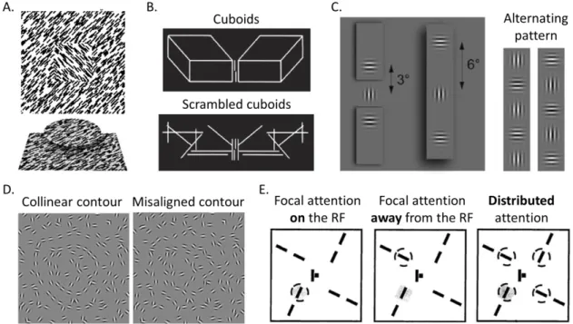
discussed below to highlight the effect of global characteristics on the contextual modulation in V1. First, Lamme (1995) showed that given the identical pattern of textured stimuli, the recorded activities from V1 neurons were determined by figure-ground segregation cues outside their RFs (as shown in Figure 1.1A). Zipser, Lamme, and Schiller (1996) further demonstrated that apart from orientation- and motion-defined figures, the segregation due to other cues, such as binocular disparity, color and
luminance, or even the combination of these cues, evoked very similar modulations in V1 neurons. The invariance in response to diverse cues suggests that the neurons are likely to respond to the higher-level perception of the “figure” generalized across multiple cues, instead of responding to a particular local feature.
The second set of studies indicates that even similar contextual stimuli may not produce similar effects at all, and it highly relies on perceptual grouping or segmentation over the scene. For example, the vernier-offset discrimination is degraded when the vernier stimulus is flanked by two lines or by multiple scrambled line segments, but the reduction can be largely recovered if those segments form a sensible object, e.g. cuboids as shown in Figure 1.1B (Herzog & Fahle, 2002; Herzog & Koch, 2001; Herzog,
Thunell, & Ögmen, 2015; Sayim, Westheimer, & Herzog, 2010). Here, if the contextual flankers are grouped with other stimuli rather than the vernier target, the contextual effect would be disrupted. Similarly, Joo and Murray (2014) showed that the orientation
sensitivity of the contextual suppression in early visual areas was observed when the center and flankers were grouped on the same surface even with a large distance between them, but not when the center and flankers were assigned to different surfaces (see Figure 1.1C (left), also see Huang, Chen, and Tyler (2012) for an example with collinear
facilitation). Interestingly, if the center and flankers jointly form an alternating pattern (Figure 1.1C (right)), the contextual suppression would be very strong (Joo, Boynton, & Murray, 2012). In all the examples, the visual perception and early visual cortical
responses to the center target are influenced by a much larger context, and are modulated by perceptual grouping/segmentation.
The perceptual state, visual attention and learning can also modulate the effects of context. Zipser et al. (1996) used dichoptic presentations of the figure-ground textures (Figure 1.1A) and demonstrated that even with a large change in the stimulus, if it had little perceptual effect, it would not alter the neuronal responses in V1 either; that is, the contextual modulation correlated with perceptual experience but not physical visual inputs. Altmann, Bülthoff, and Kourtzi (2003) also showed that the cortical responses in early visual areas could be very similar to the collinear contours (Figure 1.1D (left)) and to the perceptually detected but in fact misaligned contours (Figure 1.1D (right)).
Additionally, attention and perceptual learning play an important role in modifying V1 contextual modulation. When the attention is distributed to multiple locations, a larger increase in the response to the target (with flanker) is observed comparing with the condition with the focal attention on the RF; but this effect could be diminished by learning/overtraining (Gilbert, Ito, Kapadia, & Westheimer, 2000; Minami Ito & Gilbert, 1999; Minami Ito, Westheimer, & Gilbert, 1998).
Figure 1.1. Example studies highlighted the effect of global characteristics on the contextual modulation in V1. A. orientation-defined (above) or binocular disparity-defined (below) figure-ground segregation, adapted from Lamme (1995) and Zipser et al. (1996). B. The vernier stimulus surrounded by cuboids or scrambled cuboids, adapted from Sayim et al. (2010). C. Left, the center and flankers on different surfaces or the same surface, adapted from Joo and Murray (2014). Right, an alternating pattern jointly formed by the center and flankers, adapted from Joo et al. (2012). D. Collinear and misaligned contours among background clutter, adapted from Altmann et al. (2003). E. The target line segment with flanker presented with focal attention on the RF, away from the RF, or attention distributed among all targets. The attention is illustrated using dashed circle, and shaded region indicates the RF, adapted from Gilbert et al. (2000).
higher-level areas to influence the responses at lower levels. What would be the
underlying structure allowing such dedicated process? Visual processing is hierarchical in primates with a sequence of areas in which individual neurons access visual inputs from increasingly large regions and process increasingly complex forms of visual inputs (Felleman & Van Essen, 1991; Markov & Kennedy, 2013; Wallisch & Movshon, 2008). The first stage of visual processing happens in the retina, and the signals are then passed to the lateral geniculate nucleus (LGN), to primary visual cortex (V1) and the second visual area (V2), and then to the extrastriate areas of the dorsal and ventral streams. Areas in the dorsal stream, such as middle temporal complex (MT+) and V3 accessory (V3A), are involved in the processing of visual motion; and ventral areas, such as V4 and lateral occipital complex (LOC), are thought to represent complex visual patterns and objects (DeYoe, Felleman, Van Essen, & McClendon, 1994; Ungerleider & Haxby, 1994). Besides these feedforward connections in cortex, each cortical area receives strong feedback connections from multiple areas: in most cases where there is a forward projection from one area to another, there is a projection in the opposite direction (Felleman & Van Essen, 1991; Markov et al., 2013). The feedback connections provide infrastructure that would permit early visual areas access to perceptual interpretations of the visual scene, such as figure-ground segregation, surface representations and
perceptual grouping, from higher-level cortical areas.
Modulations from regions outside the classical RF of neurons either through the intra-areal or inter-areal connections in fact serve as a general rule at various levels in the visual system (Allman, Miezin, & McGuinness, 1985). Exploring the source of these
modulations would allow us a better understanding of the perceptual organization and its processes. In this thesis, focusing on contextual modulations in early visual areas yielded at both local and global levels, we study the role of context in shaping cortical responses and the fundamental goal of the contextual effects on visual perception.
1.2 Major questions and structure of the thesis
With a series of experiments, Murray, Kersten, Olshausen, Schrater, and Woods (2002) demonstrated an opposite response pattern between the lateral occipital complex (LOC) and primary visual cortex (V1) suggesting contextual effects in early visual areas are influenced by grouping processes in higher-level areas. Specifically, cortical response increases in the LOC and concurrent response decreases in V1 are observed when
coherent shapes are formed by line segments or by coherently moving dots (also see Händel, Lutzenberger, Thier, and Haarmeier (2007), Dumoulin and Hess (2006), Paradis et al. (2000) and Cardin, Friston, and Zeki (2010) for similar results in V1). However, other studies show response enhancement in V1 to coherent structure relative to
scrambled elements (Altmann et al., 2003; Bauer & Heinze, 2002; M. Chen et al., 2014; Kourtzi, Tolias, Altmann, Augath, & Logothetis, 2003; W. Li, Piëch, & Gilbert, 2006; McManus, Li, & Gilbert, 2011; Roelfsema, Lamme, & Spekreijse, 2004); or no
sensitivity to structure or motion coherence is observed in V1 (Kriegeskorte et al., 2003; Peuskens et al., 2004). Why does visual context at times suppress, enhance, or have no effect on cortical responses in early visual areas? In Chapter 2 and Chapter 3, two sets of experiments considering context at a more global level are used to reconcile competing branches of the literature in terms of the V1 cortical response patterns to detection of
visual structure. These results reinforce the importance of visual context in modulating responses in early visual areas.
If contextual modulation is a general process at various levels of the visual system, what are the fundamental purposes or what are the basic rules the process needs to follow? In Chapter 4 and Chapter 5, two sets of psychophysical experiments use the tilt illusion and the shape distortion, respectively, as probes to explore the functions of local and global context and to discuss their ecological meaning to visual perception. Overall, such process ensures the system would dynamically adjust weights between an efficient representation in lower-level areas and a strategy to emphasize targets and to indicate certainty. Additionally, a stronger perceptual grouping cue between the center and surround or a larger uncertainty to the center target would enhance the contextual modulation and increase perceptual biases, which would potentially increases the visual system sensitivity to feature discrepancies, or to features otherwise easily confused or degraded. Chapter 6 summarizes the work of this thesis, and future directions are proposed.
2.
The effect of global shapes in structure-from-motion perception
2.1 Introduction
Structure-from-motion (SFM) is the perception of three-dimensional structure derived from projected two-dimensional motion of segments (Wallach & O'Connell, 1953). For example, stimuli composed of two-dimensional (2D) moving dots can be perceived as objects rotating in depth (Andersen & Bradley, 1998). Both lesion studies and electrophysiological recordings demonstrated that middle temporal area (MT) plays an essential role in SFM percepts (Bradley, Chang, & Andersen, 1998; Dodd, Krug, Cumming, & Parker, 2001; Newsome & Pare, 1988; Siegel & Andersen, 1990), while functions in the area V1 may be modest (Grunewald, Bradley, & Andersen, 2002). Using functional magnetic resonance imaging (fMRI) in humans, the SFM perception-relevant network has been demonstrated to extend dorsally into the middle temporal complex (MT+) and the parieto-occipital junction (V3A) and ventrally into object-sensitive regions, such as LOC (Kriegeskorte et al., 2003; Orban, Sunaert, Todd, Van Hecke, & Marchal, 1999; Paradis et al., 2000; Peuskens et al., 2004; M. E. Sereno, Trinath, Augath, & Logothetis, 2002; Todd, 2004).
Receptive fields in V1 limit the field of view of a neuron to just a portion of the moving dots (usually smaller than 2 degree in diameter), and hence, it is not possible for one neuron in V1 to signal with certainty the true structure of the object in a purely bottom-up manner. Comparing with area V1, area MT has neurons with large receptive
fields. It is, therefore, capable of spatially integrating motion cues across large angular subtense, about 5-10 degrees (Adelson & Movshon, 1982; Albright & Desimone, 1987; J. A. Movshon, Adelson, Gizzi, & Newsome, 1985; J. A. Movshon & Newsome, 1996); it is also able to distinguish coherent versus incoherent motion (Cheng, Fujita, Kanno, Miura, & Tanaka, 1995; McKeefry, Watson, Frackowiak, Fong, & Zeki, 1997). In addition, area MT is important in tasks of transforming motion cues into information about surfaces and depth (Born & Bradley, 2005; Hildreth, Ando, Andersen, & Treue, 1995; Maunsell & Essen, 1983a, 1983b; McLeod, 1996; Orban, 1997; A. W. Roe, Parker, Born, & DeAngelis, 2007; Snowden, Treue, Erickson, & Andersen, 1991; Treue,
Andersen, Ando, & Hildreth, 1995). These characteristics of area MT establish its key role in SFM percepts.
Additionally, areas V3A, V3B, and human V4 (hV4) are recognized as regions at intermediate level in the visual processing hierarchy. Both V3A and V3B are thought to be involved in processing motion information (A. T. Smith, Greenlee, Singh, Kraemer, & Hennig, 1998; Tootell et al., 1997); whereas hV4 in the ventral stream is sensitive to complex visual forms, such as high curvature and partially occluded forms (Bushnell, Harding, Kosai, & Pasupathy, 2011; Nandy, Sharpee, Reynolds, & Mitchell, 2013; Pasupathy & Connor, 2002). Further, area LOC is specialized in cue-invariant structure perception (Fang, Kersten, & Murray, 2008; Grill-Spector, Kourtzi, & Kanwisher, 2001; Grill-Spector, Kushnir, Edelman, Itzchak, & Malach, 1998; Grill-Spector, Kushnir, Hendler, et al., 1998; Gross, Rocha-Miranda, & Bender, 1972; Haxby et al., 2001;
Kourtzi & Kanwisher, 2000, 2001; Logothetis & Sheinberg, 1996; Moore & Engel, 2001; Tanaka, 1996), which is an important component in SFM percepts as well.
Response increases to coherent versus scrambled structure in higher-level areas are almost certain among existing literature, but response patterns in early visual areas often vary in different studies. For example, with spectral analysis in a MEG study, the component attributed to areas including MT increased linearly with motion coherence; while another component from early visual cortex showed the inverse dependence on motion coherence (Händel et al., 2007). Similarly, Paradis et al. (2000) and Murray et al. (2002) observed response reduction in area V1, but response increase in area LOC using fMRI when coherent SFM stimuli were presented. However, other results showed that early visual areas responded approximately equally to moving dots (Kriegeskorte et al., 2003).
In order to reconcile these results, two levels of contextual modulations were considered in the current study. At the first level, the motion coherence was controlled, so either coherent structures or scrambled-dot motion would be perceived. At the second level, the familiarity of the perceived shapes was manipulated. In both cases, local stimulus features such as motion vectors and texture gradients of the moving dots were largely maintained to ensure that area V1 receives similar ascending signals, and thus modulations in V1 activity were most likely attributed to long-range horizontal connections or inter-areal feedback.
Two functional imaging experiments were conducted using SFM stimuli with either unfamiliar/complex (Experiment 1) or simple (Experiment 2) structures. Two
conditions were included within each experiment: in the coherent condition, transparent three-dimensional (3D) structures rotating in depth could be perceived; in the scrambled condition, motion coherence and opponent 2D motion are maintained but no 3D structure can be perceived. In both experiments, area V3A/B and LOC showed significant
preference to the coherent structure; however, the response reduction in V1 was only observed in Experiment 2 when the structure is simple. These results suggest that both local and global context would influence cortical responses in early visual areas. 2.2 Methods
2.2.1 Participants
Eight observers (mean age: 30 years old, four males) and five observers (mean age: 28 years old, three males) with normal or corrected-to-normal visual acuity participated in Experiment 1 and Experiment 2, respectively. The observers provided informed written consent under an experimental protocol that was in accordance with safety guidelines for MRI research and was approved by the Institutional Review Board at the University of Minnesota.
2.2.2 Visual stimuli
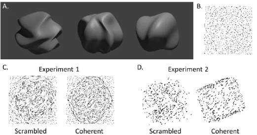
Experiment 1. Novel 3D structures were generated using perturbations in spherical harmonics (Figure 2.1A). The 3D positions of the dots were randomly selected over the structure surface, and were presented under parallel projection. The projected dots would sometimes be adjusted to ensure that the dot density was approximately uniform (Figure 2.1B). The dot trajectories were computed by projection of this set of dot positions as the structure moving in 3D. The structure was modeled as transparent with the dots
continuously visible even when they moved to the back surface. For each presentation (900 ms), the structure would rotate about a random axis in 3D space for about 40°, and the starting frame was also random.
Experiment 2. A simple structure, cube, was used to substitute the novel shapes in Experiment 1, and other parameters were maintained.
In both experiments, displays consisted of ~450 moving dots occupied about 10° visual filed. The dots were round with a radius of 0.08° visual angle. Each stimulus contained a fixation region with a diameter of 1° visual angle at the center of the screen. Two conditions, scrambled and coherent SFM, were included. Low-level stimulus features were identical for both. In the coherent SFM condition, parameters that induced stable SFM percepts based on Siegel and Andersen (1988) were applied. In the scrambled conditions, the motion vector for each dot was maintained, but the position of the dot was randomly shifted with a small amount. As a result, the perception of a coherent surface was eliminated, and, instead, a cloud of dots would be seen rotating in depth without a 3D surface or structure. In this way, local motion coherence (percentage of dots locally moving in the same direction) and opponent motion (opposite local motion direction) were well maintained. Within a small area of the stimuli, the coherent and the scrambled conditions show almost no difference. However, the perceptions of these stimuli were quite different. Figure 2.1C&D illustrate the stimuli in both experiments for scrambled and coherent conditions using a summation of three continuous frames.
Figure 2.1. Examples of stimuli used in the structure-from-motion experiments. A. Novel 3D shapes used in Experiment 1. B. One frame of the actual stimulus in Experiment 1, where low-level stimulus features were tightly controlled. C. Illustration of stimuli in Experiment 1 with a novel 3D shape. Sum of 3 continuous frames are shown to illustrate conditions at varying coherence levels. D. Illustration of stimuli in Experiment 2 with a cube.
2.2.3 fMRI experiments
Stimuli were displayed using a Sony video projector (spatial resolution of 1024 × 768 pixels, temporal resolution of 60 Hz, and mean luminance of 168 cd/m2) on a
translucent screen positioned within the scanner bore. Observers viewed the stimuli from a distance of 72 cm through a mirror located above their eyes (mounted on the head coil), which gave a total image area subtending 29.1° × 21.8°. Stimuli were presented using Matlab (R2010b; Mathworks, Inc., Natick, MA, USA) with the Psychtoolbox extensions (Brainard, 1997; Pelli, 1997). Behavioral responses were collected via a FIU-005 fiber optic response device (Current Designs, PA).
Functional MRI data were collected using a 7T scanner (Siemens, Erlangen, Germany) with a head gradient set. A sensitive gradient echo imaging pulse sequence was used: TR = 2 s, TE = 18 ms, flip angle = 70°, matrix = 108 x 108, GRAPPA
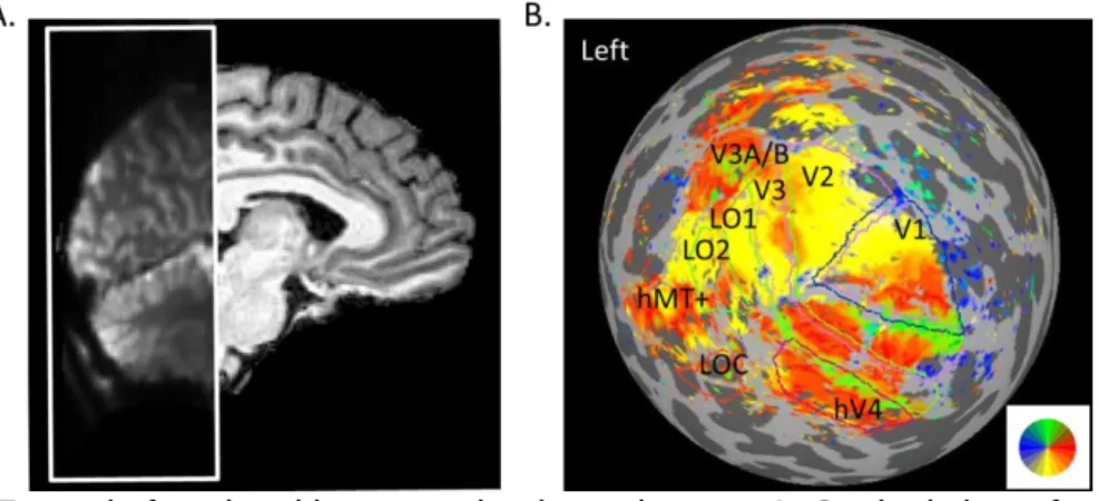
acceleration factor = 2, FOV = 162 x 162 mm, partial Fourier = 7/8, voxel size = 1.5 mm isotropic, and 36 coronal slices were obtained to cover the occipital lobes (Figure 2.2A).
A scanning session contained four runs of block-design experiments. Three conditions including scrambled/coherent SFM stimuli and a control condition with static frames were randomly interleaved. Each block lasted 16 sec, in which 16 different rotations were presented each with 1 sec (100 ms static at the end for each rotation). In the control condition, 16 random static frames were shown for each block. Observers were instructed to perform a mental calculation task at the fixation region.
2.2.4 Anatomical acquisition and visual area mapping
A T1-weighted anatomical image (sagittal MP-RAGE, 1 mm isotropic resolution)
was acquired for each participant in a separate session using a Siemens Trio 3T magnet. FreeSurfer (Dale, Fischl, & Sereno, 1999; Fischl, Sereno, & Dale, 1999) was used for segmentation, cortical surface reconstruction, and surface inflation and flattening of the anatomical image. The warped surface was then converted to a standard mesh using SUMA (Saad, Reynolds, Argall, Japee, & Cox, 2004). Visual areas were defined in a separate scanning session following standard procedures, including four runs of a clockwise/counter-clockwise rotating wedge stimulus plus two runs of an
expending/contracting ring stimulus to identify the visual areas V1, V2, V3, V3A/B, and hV4 (DeYoe et al., 1996; Engel, Glover, & Wandell, 1997; Larsson & Heeger, 2006;
Wade, Brewer, Rieger, & Wandell, 2002), two runs contrasted blocks of translating and static low-contrast dots to locate the MT+ (Tootell et al., 1995; Zeki et al., 1991), and two runs contrasted scrambled and coherent objects for LOC (Kourtzi & Kanwisher, 2001; Malach et al., 1995). Figure 2.2B shows an example angular map with identified visual areas labeled. Area V3B appeared to share the central representation with V3A (Press, Brewer, Dougherty, Wade, & Wandell, 2001; Wandell, Brewer, & Dougherty, 2005), and the boundary between the two was not clear, we would combine them as V3A/B in the analysis below.
Figure 2.2. Example functional image and retinotopic map. A. Sagittal view of example functional image coverage. The image within the white box shows a session average of pre-processed functional data. B. Example angular visual field map from a left
hemisphere (inflated cortical surface visualized as a sphere) with identified visual areas labeled.
2.2.5 Pre-processing
Motion correction parameters acquired using AFNI (Cox, 1996) with reference to the volume right before a within-session fieldmap image were first combined with distortion unwarping parameters via FSL (S. M. Smith et al., 2004). Functional imaging
data were then resampled with sinc interpolation. Individual observer’s anatomical image was aligned with a mean of all the functional images with AFNI’s align_epi_anat.py using six free parameters for translation and rotation. Please see Mannion, Kersten, and Olman (2014) for more details. The pre-processed functional data were then projected onto the standardized cortical surface. All analysis was performed on the nodes of this surface domain representation.
2.2.7 Analysis
A general linear model (GLM) was used to analyze the functional data. Stimulus blocks for each condition were modeled as boxcars and convolved with SPM’s canonical hemodynamic response function. The GLM was estimated using AFNI’s 3dREMLfit, which estimates and removes noise temporal correlations with a voxelwise ARMA(1,1) model. The stimulus condition beta estimates for each node from the GLM were
converted to percent signal change via division by the estimate baseline timecourse from nuisance regressors. These percent signal change values were than averaged across the nodes that significantly responded to the moving conditions within each predefined visual area. Results were normalized to the control (static) condition for each experiment. Statistical significance for BOLD response differences between conditions was assessed using a bootstrap procedure in which observers’ data were resampled with replacement across 10000 iterations. The p-values (two-sided test) were corrected using Bonferroni procedure.
2.3 Results
The surface nodes responsive to the moving conditions were first identified (within the ~10° central visual filed). In detail, for each observer, the nodes with a
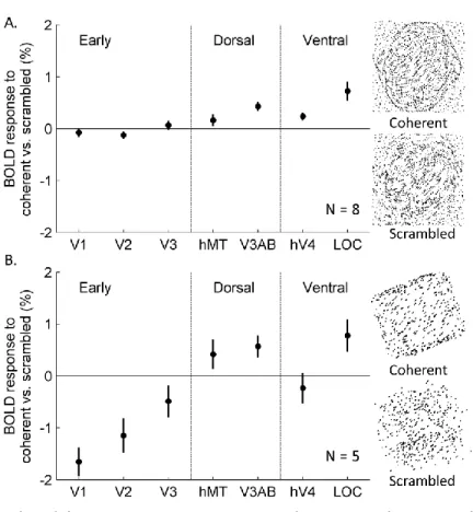
significantly positive ( , hemisphere FDR corrected) coefficient for the contrast between the sum of the response to moving stimuli and the response to the static control stimuli were selected. The responses to the coherent and scrambled SFM stimuli were then averaged within selected nodes of each predefined visual area. The BOLD response differences between the two conditions are shown in Figure 2.3 for both experiments. A positive number indicates a stronger response to the coherent condition than the
scrambled, and a negative number shows a preference to the scrambled condition. Among the early visual areas, V1 and V2 showed significant modulations only in Experiment 2 with the Bonferroni adjusted (bootstrap two-sided test) for both areas, and the mean response difference was -1.65% in V1 and -1.15% in V2. In contrast, the uncorrected p-values in area V1 and V2 in Experiment 1 were 0.176 and 0.036, respectively. For dorsal regions, V3AB showed a significant response increase to the coherent SFM condition in both experiments with corrected , and the response difference was 0.43% in Experiment 1 and 0.57% in Experiment 2. MT+ had a weak preference to the coherent condition in Experiment 2 (corrected with mean response difference 0.42%). In ventral areas, hV4 revealed slight but consistent response increase (mean as 0.24%, corrected ) to the coherent condition in Experiment 1; LOC showed strong preference to the coherent condition in both experiments
Figure 2.3. Results of the BOLD response contrast between coherent and scrambled SFM stimuli. A. Results from Experiment 1 when the structures are novel 3D shapes generated using perturbations in spherical harmonics. B. Results from Experiment 2 when the structure is a cube. Error bars show ±1 SE.
2.4 Discussion
We investigated how global structure context would affect the responses in human visual cortex (early visual areas and some dorsal/ventral areas) using fMRI. Our results show that the effect of motion coherence would also be modulated by the global shape. In Experiment 2, we replicated the response reduction in early visual areas (V1 and V2) when a coherent simple cube was perceived; however, no similar effect was observed in Experiment 1 when the novel 3D structures were presented.
Murray et al. (2002) proposed a possible explanation for the response reduction in V1 with coherent perception: the predictive coding theory (Mumford, 1992; Rao & Ballard, 1999) would predict such reduction due to the decrease of unexplained residuals in V1 when visual inputs were successfully modeled as coming from a coherent shape. Our results would argue that the reduction is selective: given an easy target, though the constant lower-level inputs are suppressed, the structure still could be accurately
represented in the high-level areas; whereas when the perceived shape was complicated, though the structure had already been sensed by the higher-level areas (such as LOC), constant lower-level inputs were still necessary for the system to encode the novel shape.
Area hV4 also appeared to be sensitive to the shape familiarity, in which a significant preference to the coherent structure was observed in Experiment 1 but not in Experiment 2. More resources were engaged when the visual structure was complex or unfamiliar. In contrast, area MT+ was less responding to the shape information: it equally responded to both moving conditions in Experiment 1, and only showed a weak trend in preferring coherent structure in Experiment 2.
Additionally, we found that V3A/B may be at a higher hierarchical level than MT+ in the dorsal stream because of a more consistent preference for coherent SFM in V3A/B than MT+, and this hierarchy is also anatomically predicted by Markov et al. (2013). A similar relationship has been demonstrated between ventral areas hV4 and LOC: hV4 is selective to intermediate-level features, whereas LOC responds to global shapes (Kourtzi & Kanwisher, 2001; Lerner, Hendler, Ben-Bashat, Harel, & Malach, 2001; Pasupathy & Connor, 2002). In our results, both V3A/B and LOC had more
consistent preference to coherent moving structures independent on familiarity, suggesting their crucial role in global shape representations. This result was in fact consistent with many studies that have reported greater sensitivity to 3D surface in V3A (Grill-Spector et al., 2001; Grill-Spector, Kushnir, Edelman, et al., 1998; Grill-Spector, Kushnir, Hendler, et al., 1998; Paradis et al., 2000; M. E. Sereno et al., 2002).
To summarize, we have shown that the responses of human early visual areas to structures relying on both their coherence levels and global shape familiarity. This ensures the system flexibility to switch or dynamically weight between strategies to both efficiently and accurately represent visual inputs.
3.
Responses in early visual areas to contour integration are context
dependent
Authors
Cheng Qiu, Philip C. Burton, Daniel Kersten, Cheryl A. Olman Summary
It has been shown that early visual areas are involved in contour processing. However, it is not clear how local and global context interact to influence responses in those areas, nor has the inter-area coordination that yields coherent structural percepts been fully studied, especially in human observers. In this study, we used functional Magnetic Resonance Imaging (fMRI) to measure activity in early visual cortex while subjects performed a contour detection task in which alignment of Gabor elements and background clutter were manipulated. Six regions of interest (two ROIs, containing either the cortex representing the target or the background clutter, in each of areas V1, V2, and V3) were predefined using separate target versus background functional localizer scans. The first analysis using a general linear model (GLM) showed that when background clutter was absent, responses in V1 and V2 target ROIs were suppressed by aligned contours compared with unaligned, whereas in the presence of background clutter, responses were significantly stronger to aligned than unaligned contours. The second analysis using inter-area correlations showed that with background clutter, there was an increase in V1-V2 coordination within the target regions when perceiving aligned versus unaligned contours; without clutter, however, correlations between V1 and V2 were
similar no matter whether aligned contours were present or not. Both the average response magnitude and the connectivity analysis suggest different mechanisms support contour processing with or without background distractors. Coordination between V1 and V2 may play a major role in coherent structure perception, especially with complex scene organization.
Keywords: contour integration, fMRI, early visual areas 3.1 Introduction
Contour integration involves grouping local features across several levels of abstraction and a range of spatial scales. Small, similar elements positioned closely along an invisible smooth path are perceptually organized as due to a continuous contour. This grouping process is enhanced if the elements have orientations that align with the path (Field et al., 1993; Hess & Field, 1999; Kovács, 1996; W. Li & Gilbert, 2002). Further, knowledge of the global form of the path contributes to local integration, such as the form closing (Kovács, 1996; Kovács & Julesz, 1993, 1994) and smoothness (Pettet, 1999; Pettet, McKee, & Grzywacz, 1998), and the global knowledge is often necessary to disambiguate competing local groupings in cluttered scenes (Ullman & Sha'ashua, 1988).
It has been repeatedly reported that cortical areas higher in the visual hierarchy such as the lateral occipital complex (LOC) and inferotemporal cortex (IT) show selectivity to coherent contours (Altmann et al., 2003; Cardin et al., 2010; Dumoulin, Dakin, & Hess, 2008; Dumoulin & Hess, 2006; Kourtzi et al., 2003; Mendola, Dale, Fischl, Liu, & Tootell, 1999; Murray et al., 2002; Tanskanen, Saarinen, Parkkonen, & Hari, 2008), which is also consistent with results of shape or object perception from those
al., 1998; Grill-Spector, Kushnir, Hendler, et al., 1998; Gross et al., 1972; Haxby et al., 2001; Kourtzi & Kanwisher, 2000; Logothetis & Sheinberg, 1996; Tanaka, 1996). However, responses to similar contour stimuli in early visual areas are still controversial. While most neurons in the primary visual cortex (V1) are thought to have small receptive fields, it is known that their responses are modulated by contextual information from outside their receptive fields (Allman et al., 1985; Fitzpatrick, 2000). However, there are substantial conflicting results on how scene context or global perception affects responses in early visual areas, including V1.
Both enhancement (Altmann et al., 2003; Bauer & Heinze, 2002; M. Chen et al., 2014; Kapadia et al., 1995; Kourtzi et al., 2003; W. Li et al., 2006; McManus et al., 2011; Roelfsema et al., 2004) and suppression (Cardin et al., 2010; Dumoulin & Hess, 2006; Murray et al., 2002; Murray, Schrater, & Kersten, 2004) of cortical responses to coherent contours relative to scrambled elements have been observed in V1 and/or other early visual areas. Recording from individual V1 neurons in monkeys, Kapadia et al. (1995) and W. Li et al. (2006) showed that multiple randomly placed and oriented line segments outside the neuron’s receptive field would inhibit its response to an optimally oriented line within its receptive field; however, once some of the surround segments were placed collinearly with the central line, the response was then facilitated. Similar results have been demonstrated using functional neuroimaging in both monkeys and human subjects (Altmann et al., 2003; Kourtzi et al., 2003): cortical responses from early visual areas including areas V1, V2, and V3 showed selectivity to coherent patterns of closed contours embedded in a field of randomly oriented segments.
In contrast, Cardin et al. (2010) showed lower activity in areas V1/V2 for collinear patterns than for noncollinear ones. Dumoulin and Hess (2006) also showed weaker activity in early visual areas to a 100% coherence circular pattern but stronger activity to scrambled patterns. In a third study, Murray et al. (2002) used line-drawings as stimuli and showed smaller responses in V1 to lines that formed two-/three-dimensional shapes than random lines. These were not the only results showing deactivation in early visual areas to stimulus regularities – early visual areas also respond less to coherent than incoherent motion (Händel et al., 2007; Harrison, Stephan, Rees, & Friston, 2007;
McKeefry et al., 1997). A similar trend has been observed with coherent versus
scrambled natural images using functional imaging in human observers (Grill-Spector, Kushnir, Hendler, et al., 1998; Lerner et al., 2001; Paradis et al., 2000).
We are interested in how the enhancement and suppression of cortical responses in early visual areas to coherent contours could both be true. In either case, neurons in V1 are responding to the same coherent circular contour, but they show different response patterns based on different studies listed above. We think the response pattern may highly depend on stimulus context: results showing response increase mainly used contours embedded in clutter (i.e., with randomly orientated and placed segments in the
background), but the ones showing a decrease were usually using isolated structure or if any, with just uniform background. To test this, we designed a two-by-two experiment where context and contour coherence were manipulated, and we used fMRI to record the Blood Oxygenation Level-Dependent (BOLD) signal from the retinotopically
contour detection task in the experiment. When there was no background clutter present, the BOLD responses in regions corresponding to the location of the target were
suppressed by aligned contours compared with the unaligned; however, with background clutter, the response trend was reversed. By analyzing the effect of context and contour coherence on correlations between responses in early visual areas, we further
demonstrated that the coordination between the retinotopically relevant regions in V1 and V2 was dependent upon the experimental conditions. These results suggest the
involvement of multiple strategies in contour integration, and they interact according to the context.
3.2 Materials and methods 3.2.1 Participants
Twelve observers (mean age: 29 years old, seven males) with normal or corrected-to-normal visual acuity participated in the study. The observers provided informed written consent under an experimental protocol that was in accordance with safety guidelines for MRI research and was approved by the Institutional Review Board at the University of Minnesota.
3.2.2 Stimuli
Figure 3.1 provides examples of the stimuli used, which were generated and presented with Matlab (R2010b; Mathworks, Inc., Natick, MA, USA) using the
Psychtoolbox extensions (Brainard, 1997; Pelli, 1997). The target region consisted of 8 Gabor patches, which were centered at equal intervals along the circumference of an invisible circle centered at fixation with a radius of 2°, that is, these patches were evenly
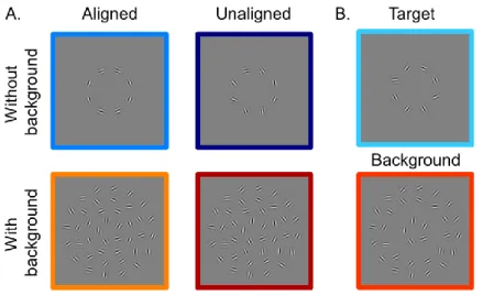
spaced at 2° eccentricity from the fixation. Each Gabor patch consisted of a 4 cycles-per-degree (cpd) sinusoidal grating with a random phase offset modulated by a Gaussian envelope with full width at half-maximum of 0.4° (σ=0.17°). In an aligned condition, the grating orientation of each Gabor patch was aligned with the tangent line to the invisible circle at the point of patch center. These Gabor patches therefore could be perceived as forming a complete circle. In an unaligned condition, the grating orientation of each Gabor patch was randomly generated. The background clutter consisting of the same Gabor elements as the target was located along invisible circles centered at fixation and with radii of 1.2°, 2.9° and 4.0°. Along each circle, the distance between every two Gabor patches was the same as in the target region (1.6°), thus the numbers of Gabor patches along each eccentricity were 5, 12 and 16, respectively. The grating orientations of these background patches were randomly generated. All Gabor patches had an 80% Michelson contrast and were presented on a mean gray background. The four experimental
conditions included aligned target only, unaligned target only, aligned target with background and unaligned target with background.
Figure 3.1 Example stimuli. A. Example stimuli from the four test conditions with a circular contour detection task. B. Example stimuli from the target (above) versus background (below) differential localizer scan.
3.2.3 fMRI experiments
Stimuli for the first four subjects were presented on a NEC 2190UXi monitor with resolution of 1024 × 768 pixels and a refresh rate of 60 Hz. The monitor had a mean luminance of 110 cd/m2. The monitor was mounted to the back wall of the scanning suite; observers viewed the monitor through a mirror mounted to the top of the head coil so that it subtended 12° of visual angle in the horizontal direction and 9° in the vertical direction. For the rest of the observers, stimuli were back-projected via a Sony video projector (spatial resolution of 1024 × 768 pixels, 60 Hz refresh rate and 120 cd/m2 mean
luminance) on to a translucent screen placed inside the scanner bore. Observers viewed the stimuli from a distance of 97.5 cm through a mirror located above their eyes
Functional MRI data were collected using a 3T Siemens Trio scanner (Erlangen, Germany) with a 12-channel head array coil. EPI data were acquired with a field of view 128 mm × 256 mm and a matrix size of 64 × 128 for an in-plane resolution of 2 mm × 2 mm. Slice thickness was 2 mm without inter-slice gap, and number of slices was 20. Echo time (TE) was 30 ms, repetition time (TR) was 1.5 s, and flip angle was 80°. Four out of the twelve datasets were collected in an axial direction, and the other eight were in a coronal orientation. Both covered the early visual areas V1, V2, and V3.
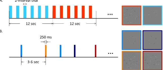
A scanning session (Figure 3.2A) contained three runs (run 1, 5 and 8) of block-design functional localizers and five event-related runs (run 2, 3, 4, 6 and 7). Observers were instructed to maintain their fixation on a white square at the center while performing behavioral tasks during both localizer and event-related scans. Behavioral responses were recorded using a fiber-optic button box (Current Designs, Philadelphia, PA, USA).
Figure 3.2. Experimental procedure. A. An example of block-designed functional
Regions of interest (ROIs) were defined by block-designed functional localizer scans (Figure 3.2A). Each block lasted 12 s, and each run contained 11 “on” blocks alternating with 10 “off” blocks. Each localizer scan thus lasted 252 s. During “on” blocks randomly oriented Gabor patches at the target region were presented; during “off” blocks only clutter Gabor patches at the background region were presented. The first half-cycle “on” block was discarded before analysis, and the remaining blocks were
alternating in 10 cycles per run. During each block, a two-interval trial occurred every 2 s (six trials per block). Duration for both intervals was 200 ms, which were separated by a 200 ms inter-stimulus interval (ISI). Observers were instructed to press button when the stimuli from two intervals were the same (with a probability of 12.5%). The fixation square turned green to a correct response and red otherwise.
The event-related runs (Figure 3.2B) measured BOLD response to four
experimental conditions: aligned target only (alnb, aligned/no background), unaligned target only (uanb, unaligned/no background), aligned target with background (albg) and unaligned target with background (uabg). Stimulus duration was 250 ms, and inter-trial intervals (ITIs) were 3, 4.5, or 6 s. ITI was randomly assigned and uniformly distributed. Each run included 20 trials for each condition, thus a total of 80 trials per run. The average run length was about 380 s. Observers were required to press the blue button if they perceived an aligned circle, and press the red button if not. Feedback was provided after each trial.
Prior to the fMRI experiments each observer participated in a separate retinotopic mapping session, in which a T1-weighted anatomical image (MP-RAGE, 1 mm isotropic
resolution) was also collected for anatomical reference and cortical surface definition. Gray/white matter segmentation, cortical surface reconstruction, and surface inflation and flattening were completed using FreeSurfer (Dale et al., 1999; Fischl et al., 1999).
Standard retinotopic mapping including four runs of clockwise/counterclockwise rotating wedges and two runs of expanding/contracting rings (DeYoe et al., 1996; Engel et al., 1997; M. I. Sereno et al., 1995) was used to identify the early visual areas V1, V2, and V3. Defined visual areas were registered to the reference anatomy for each observer. 3.2.5 Pre-processing and functional localizers
Functional data was motion corrected using Analysis of Functional NeuroImages software (AFNI) (Cox, 1996), with reference to the volume right before a within-session fieldmap image. The motion-corrected data was unwarped using FSL FUGUE to correct distortions introduced by magnetic field inhomogeneities (S. M. Smith et al., 2004). High-pass filtering was also applied to the functional localizers data: temporal
frequencies below four cycles per run were removed. The pre-processed functional data were then aligned to anatomical reference data using mrAlign implemented in Matlab (http://gru.brain.riken.jp/doku.php/mrTools/overview).
ROIs were defined based on both retinotopic visual areas and functional localizers for each observer. Three repetitions of the functional localizers were averaged to define the ROIs responding to the target (tg) or background (bkgd) regions. For each voxel coherence (unsigned correlation, computed in the Fourier domain as the amplitude of the
stimulus-related Fourier component normalized by the square root of the integrated power spectrum) with a sinusoid at the block-alternation frequency, 10 cycles per run, was calculated in the averaged localizer scans (Bandettini, Jesmanowicz, Wong, & Hyde, 1993; Engel et al., 1997). The voxels with coherence exceeding 0.30 were included in the ROIs. The voxels in phase with the target representation were assigned to target ROIs (tgROIs), and the voxels in phase with the background representation were assigned to background ROIs (bkgdROIs). ROIs were initially defined on a flattened cortical surface, where V1, V2 and V3 boundaries could be used to identify the ROIs in different visual areas. Selected voxels were translated to the in-plane space for further refinement to
include only contiguous clusters of visually responsive voxels, and the defined ROIs were then exported as a binary mask in the space of the functional data. Six ROIs were defined for each observer: tgV1, tgV2, tgV3, bkgdV1, bkgdV2, and bkgdV3.
3.2.6 Analysis of the event-related data
fMRI data analysis
Functional image analysis of the event-related runs was conducted using general linear model (GLM) in AFNI with the function 3dDeconvolve. The BOLD response to individual events from each stimulus condition was modeled using the sum of “TENT” basis functions – a piecewise linear spline function that estimates an impulse response function. The sum of 13 tent functions was used to cover the duration of 18 s after the stimulus onset (“TENT(0, 18, 13)”). All models were fit separately to each voxel. For each voxel within the pre-defined ROIs 13 amplitudes for each stimulus condition were estimated, which were the time course of the estimate hemodynamic response function
(HRF) to each condition at the 13 time points (from 0 to 18 s with the time step of 1.5 s). The mean of the first and last two time points was subtracted from each HRF to ensure that it started from and returned to approximately the same baseline level. Estimates from individual voxels were averaged within each of the 6 ROIs, and BOLD response
amplitudes were estimated using the difference between the peak response (reached around 4.5 – 6 s after stimulus onset) and the baseline response. Our analysis focused on response differences between contour aligned and unaligned conditions, instead of direct comparison between aligned or unaligned contours in clutter versus not, to avoid
confound of blood stealing from the background stimulus. Response differences between conditions were assessed using a bootstrapping procedure – resampling 12 subjects data with replacement within conditions and calculating differences across 10000 iterations, and a one-sided permutation test was performed to acquire p-values (Efron & Tibshirani, 1993). Analysis of variance (ANOVA) was also conducted to compare BOLD response amplitudes among conditions in each predefined ROI.
Connectivity analysis
Besides the estimated response to each stimulus condition, we also wanted to know whether interregional connections among these ROIs depend on the experimental conditions. Two functional connectivity analysis methods were used to answer this question. The first method, psychophysiological interactions (PPI), uses interaction terms created from the dot product of the seed region time series and vectors representing different experimental conditions to explain variance in time series from other cortical regions with a GLM analysis. If the estimated beta weights for the interaction regressors
are different among experimental conditions, the coordination between the test ROI and the seed ROI depends on the conditions. In the second method, beta series correlations, a beta weight for each experimental trial is estimated using GLM, these beta weights are sorted according to the experimental condition during the trial, and then correlations are calculated between the beta weights for each condition (Rissman, Gazzaley, &
D'Esposito, 2004). If these correlations vary depending on the conditions, connectivity between the two regions is condition-dependent.
Psychophysiological interactions. First, the data modeled by the GLM (driving
effect of stimuli) was subtracted from the pre-processed event-related dataset to generate a residual dataset for further analysis of the intrinsic interactions between cortical areas. Figure 3.3 shows an example of the PPI terms (regressors in a GLM). In order to build the psychophysiological interaction terms, both psychological condition codes (indicating the representation time for a certain stimulus condition) and physiological responses from the seed region (selected based on the BOLD response modulation across conditions) were required. According to McLaren, Ries, Xu, and Johnson (2012), with more than two conditions separately building one interaction term for each stimulus condition could be more robust to noise and have better model fits than directly using PPI terms with condition contrast (i.e., “1” for one condition while “-1” for a different condition). Therefore, we created one text file matching the length of functional time series for each condition as the condition code ( ), in which “1” indicated stimulus presentation of that particular condition and “0” for the rest time points (Fig. 3B right panel). The
series from the seed region with its HRF estimated from the previous analysis (Fig. 3A). Gitelman, Penny, Ashburner, and Friston (2003) and Kim and Horwitz (2008)
demonstrated the importance of modeling the underlying neural activity: interaction should be expressed at a neuronal level rather than at the level of hemodynamic responses – neuronal activity being filtered with an HRF. Interaction was calculated as the product of condition codes and estimated physiological responses (Figure 3.3B). In order to compare the interaction with BOLD measurements, we then convolved the interaction at a neuronal level with HRFs to obtain a regressor at the level of hemodynamic responses (Figure 3.3C).
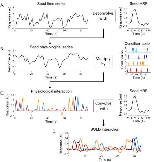
Figure 3.3 An example of the psychophysiological interactions term. A. The seed time series were first deconvolved based on the estimated HRF to obtain physiological responses. B. To combine both the physiological and psychophysical effects we multiplied the seed physiological series by the condition code from each condition separately. C. The interaction at the physiological level was convolved with the
estimated HRF, so we could compare this BOLD level interaction (as shown in D) with residual time series from other ROIs.
In summary, residual time series from the ith ROI, , could be modeled as (Friston et al., 1997):
, (*)
where c is the stimulus condition index, here, we have four conditions, ; is the correlation coefficient for the PPI regressor of condition c at ROI i; is the correlation coefficient for the seed time series regressor at ROI i; indicates the convolution operation with the estimated TENT HRF for a certain condition (c) in the corresponding region (here, the seed region); is the stimulus presentation code for condition c; is the time series from the seed region and is the physiological response estimated by deconvolving with the estimated HRF, that is, since
, we could solve for given the kernel function and using deconvolution; finally, is an error term at region i. The beta estimated for the PPI regressor represents the amount of signals could be explained by both the response in the seed ROI and the stimulus condition. If the beta estimates at a certain ROI from two conditions are different, the seed may differently influence this ROI between these two conditions. Next, 3dDeconvolve and 3dREMLfit (which estimates and removes noise temporal correlations) were used to estimate coefficients based on the model (*).
Estimates of from individual voxels were averaged within ROIs, and would be used for assessing statistical significance.
Beta series correlations. With the beta series correlation method (Rissman et al.,
2004), we first estimated a beta weight for each experimental trial, that is, modeling the time series from the ith ROI, , as
where c is the index for the stimulus conditions; i is the index for the ROIs;
indicates the estimated hemodynamic response function at the region i for the condition
c; is the beta weight for the ith ROI during the jth trial of the condition c; is the total number of trials for the condition c; is an error term at region i. Next, the estimated beta values from the ith region were regressed against the
from the region (the seed) according to the conditions, and the estimated linear coefficient was used to indicate the connectivity between regions and under a certain experimental condition.
3.3 Results
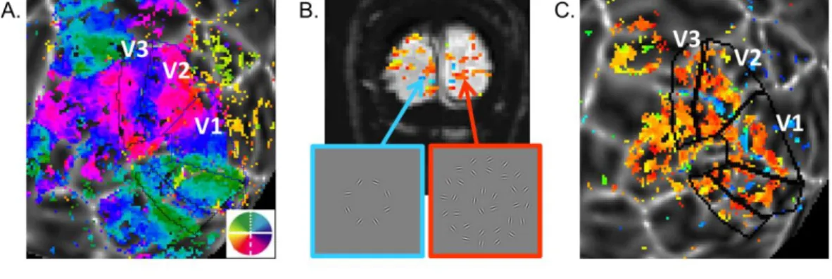
The early visual areas V1, V2, and V3 were manually defined according to the polar angle (Figure 3.4A) and eccentricity phase maps acquired in separate scanning sessions. Functional localizers (three runs, pre-processed, averaged and subjected to Fourier analysis) were used to define ROIs corresponding to the cortical representations of stimulus target or background regions (Figure 3.4B and C). On the flat patch, a band of activation associated with the target representation (blue, Figure 3.4C) and two bands associated with the background representations (orange, Figure 3.4C) were consistent with the eccentricity features in the early visual areas. Therefore, two sets of ROIs were defined in each visual area corresponding to target (tgROIs) and background regions (bkgdROIs).
Figure 3.4 Visual area mapping (A) and functional localizer results (B and C). A. Angular visual field preference of one observers’ left hemisphere obtained from rotating wedge stimulus (overlay on a flattened patch of the cortical surface centered on the occipital pole). The early visual areas are labeled. B. On one single coronal EPI image, voxels significantly correlated with the block-alternation are color coded based on relative phases – the bluish voxels are in phase with the target presentation, while the orange voxels are in phase with the background stimulus. C. Data in B was transformed to the flat patch, where a blue target-associated band and two orange background-associated bands could be seen among the early visual areas.
3.3.1 Stimulus-related activity
We first looked at the BOLD response magnitude for each experimental
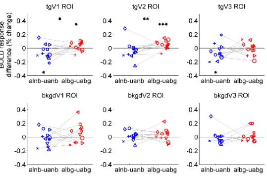
condition. Estimated HRFs in one representative subject within the tgV2 ROI are shown in Figure 3.5. The differences of BOLD responses to the aligned from the unaligned contours for each ROI depend on the background context as shown in Figure 3.6. When the background was present, the tgV2 ROI showed a significant preference for the aligned contours ( , with one-sided permutation test ). In tgV1 the responses to aligned contours were weaker than the responses to the unaligned
there was no background. Using a two-way ANOVA model within each visual area (Alignment and Background as fixed effects, and subjects as a random effect), a significant interaction between Alignment and Background was observed in tgV2 ROI
( ) and a similar trend was seen in tgV1 ROI
( ). When we tested for this interaction using a permutation test, tgV2 showed , and tgV1 showed . No significant effect was found in background ROIs. Thus, the regions in V1 and V2 corresponding retinotopically to the target ring responded to the coherent contour differently according to the context.
Figure 3.5 Estimated HRFs from four experimental conditions for one subject’s tgV2 ROI. The HRFs were estimated for each voxel, and then averaged within each ROI.
Figure 3.6 Stimulus-related BOLD response differences among conditions. Each panel shows data from one ROI for individual subjects (shown in different icons). Blue icons are differences of estimated HRF amplitudes between the aligned and unaligned contours when there was no background, and red icons are BOLD differences when there was background clutter. Gray lines connect data points from the same subject. Asterisks indicate statistical significance based on one-sided permutation test at
* , ** and *** .
3.3.2 Coordination among regions influenced by physiological and psychological states
We also explored coordination among defined ROIs using two connectivity analysis methods. With the PPI analysis, we used the tgV2 ROI, which showed strong modulations among conditions, as the seed region. The PPI connectivity results are shown in Figure 3.7. When the background was present, beta estimates for the aligned
condition were larger than the unaligned ( , with permutation test ) in tgV1 ROI. Using a two-way ANOVA model within each ROI (Alignment and Background as fixed effects, and subjects as a random effect), a significant interaction between Alignment and Background was observed in tgV1 ROI ( ). The correlation differences were also retinotopically specific to the target ROIs: no effect was observed in the background ROIs.
Figure 3.7 Connectivity results using PPI. Differences of Beta estimates among conditions are shown when tgV2 was the seed (dashed frame). Blue icons are
differences of estimated beta weights of PPI terms between the aligned and unaligned contours when there was no background, and red icons are differences when there was background clutter. Gray lines connect data points from the same subject. Asterisks show significant levels based on the permutation test.
With a second inter-area connectivity analysis, the beta series correlations, a beta value was first estimated for each experimental trial. Next, these beta values were sorted according to conditions and correlated among ROIs for each condition (Figure 3.8A). Figure 3.8B shows differences of beta series correlations estimated in tgV1 against tgV2 ROI. With the background, the linear coefficients of beta values from the tgV1 against beta values from the tgV2 were larger when the Gabors were aligned
( , with one-sided permutation test ); a weak trend of interaction between the Alignment and Background was also observed (with
permutation-based ; ANOVA, ). The ANOVA p-values of the
Alignment and Background interactions are shown in Figure 3.8C, which shows similar sensitivity to experimental conditions of tgV1-tgV2 connectivity as using the PPI analysis. A significant interaction was also observed in tgV3 when tgV2 was the seed (
), and in bkgdV3 when bkgdV2 was the seed ( ).
Figure 3.8 Connectivity results using beta series correlations.A. Scatter plot of the beta values in tgV1 against those in tgV2 for a single subject under the albg (in orange) and uabg (in dark red) conditions. B. Differences of beta series correlations estimated in tgV1