USING AN ANT COLONY OPTIMIZATION ALGORITHM FOR IMAGE EDGE DETECTION AS A THRESHOLD SEGMENTATION FOR OCR SYSTEM

5675

ACCELERATING THE OUTLIER DETECTION METHODS

FOR CATEGORICAL DATA

BY USING MATRIX OF ATTRIBUTE VALUE FREQUENCY

1_{NUR ROKHMAN,} 2_SUBANAR, 3_{EDI WINARKO}

1_{Gadjah Mada University, Department of Computer Science and Electronics, Yogyakarta, Indonesia} 2 _{Gadjah Mada University, Department of Mathematics, Yogyakarta, Indonesia}

3 _{Gadjah Mada University, Department of Computer Science and Electronics, Yogyakarta, Indonesia}

E-mail: 1_{[email protected],} 2_{[email protected],} 3_{[email protected]}

ABSTRACT

Based on the data, outlier detection methods can be classified into three classes. Those are the methods which work on numerical data, work on categorical data, and work on mixed type data. Most of the outlier detection method works on numerical data. Only few method works on categorical data or work on mixed type data. In this paper, a new method for detecting outlier in categorical data called Weighted Matrix Entropy Value Frequency (WMEVF) has been proposed. This method uses weighting function to improve the precision and uses a matrix of attribute value frequency to reduce the complexity. There are four weighting functions used in the experiments namely: range, variations, deviation standard, and square function.

The performance of WMEVF is observed based on the detected outlier of UCI Machine Learning datasets and the time needed to detect the outlier. The experiments show the fact that square function improved the precision and the matrix of attribute value frequency reduced the complexcity from O(m*n2_{) to O(m*n).}

Keywords: Outlier Detection, Categorical Data, Weighting Function, Entropy, Attribute Value Frequency.

1. INTRODUCTION

Outlier detection is an important step in data processing. Outlier detection method is used to find uncommon data. An outlier is one that appears to deviate markedly from other members of the sample in which it occurs [1]. An outlier might be generated by a different mechanism of the systems [2] and very low frequency [3]. Outliers or anomalies are patterns in data that do not conform to a well-defined notion of normal behavior [4].

Many outlier detection methods have been developed. Most of the existing methods works on numerical data. Statistical-based method, distance-based method, density-based method, and clustering-based method are the common methods for numerical data [4]-[7].

For non-numerical data, a mapping process to a numerical value is needed. Attribute Value Frequency (AVF) method uses frequency data as the numerical value [8]. Similarity-dissimilarity concept with contingency table is used to determine the graphical plot of categorical data [9]. Categorical data is converted into numerical data by using

co-occurrence theory, which explores the relationship among items to define the similarity between pairs of objects [10]. The numerical value can be used to find the outlier.

Weighted Density Outlier Detection (WDOD) method uses attribute value frequency and average density to detect outlier of categorical data [11]. Automated Entropy Value Frequency (AEVF) uses entropy change to determine the degree of outliers. The data which cause the higher entropy change have the higher degree of outliers. A complete evaluation of various mechanisms which maps categorical data into numerical data to detect outlier has been done [4].

Among of the above methods, AEVF has the best performance. AEVF method always generate the optimal number of outliers [12]. Unfortunately, AEVF suffers from its complexity. Its complexity is

O(m*n2_).

5676 Detection (WADOD) method use weighting functions to improve the performance of AVF and WDOD methods [19].

This paper discusses the construction of new outlier detection method for categorical data called Weighted Matrix Entropy Value Frequency (WMEVF). WMEVF is constructed from AEVF [12] by implementing matrix of attribute value frequency and weighting function. The matrix of attribute value frequency is used to reduce the algorithm complexity. The weighting function is used to improve the precission.

The performance of the weighting functions are observed by their effects on the capability of finding the outlier data. Three datasets from UCI Machine Learning repository, namely Mushroom,

Nursery, and Adult are used as the case study [20].

The remaining paper is organized as follow. Section 2 presents the related works. Section 3 describes the proposed algorithm. Section 4 describes the experimental setup, results, and discussions. Section 5 summarizes the discussion and future works.

2. RELATEDWORKS

There are three categories of outlier detection methods, namely: supervised, semi-supervised, and unsupervised outlier detection method. For the supervised outlier detection method, both the normal data and the outlier are labeled. The outlier detection method is used to determine whether an observed data is a normal data or an outlier. The semi-supervised outlier detection method labels only the normal data.

The uunsupervised outlier detection methods implicitly assume that: (1) normal instances are much more frequent than the outlier instances, (2) the outlier instances are far from the normal instances, (3) the normal instances are much denser than the outlier instances [4].

For the categorical data, the existing methods for detecting the outliers are: AVF [8], WDOD [11], AEVF[12], MR-AVF (Map Reduce AVF) [21], NAVF (Normally distributed Attribute Value Frequency) [22], OPAVF (One Pass Attribute Value Frequency) [23], FuzzyAVF [24], WAVF [19], and WADOD [19]. These methods work base on the attribute value frequency. AVF method is the simplest method. The AVF method is parallelized by

MR-AVF method. WDOD method uses attribute value frequency and average data density to detect the outlier. WAVF and WADOD methods use the weighted attribute value frequency to improve the precision of AVF and WDOD method. These methods belong to the unsupervised outlier detection methods.

AEVF method uses the change of entropy of value frequency. AEVF is developed from the LSA method [25] by introducing maximum entropy gap [12]. Maximum entropy gap is the average of entropy difference from the total entropy when an object is taken out from the categorical data. An outlier is an object which has entropy difference greater than the maximum entropy gap.

3. PROPOSEDALGORITHM

This section gives a detail explanation of WMEVF method. The explanation covers the construction of the WMEVF method, practical examples, and algorithm.

Definition 1. Categorical data

A categorical data can be defined as quadruple

DT=(U, A, V, f), where U is a non-empty set of the

objects, A is a non-empty set of attributes, C is a

non-empty set of the value attribute domain, and V

is the union of ∈ . : → is a function, where ∀ ∈ , ∈ , , ∈ . is the domain value of attribute a.

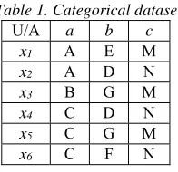
Consider the categorical data [11] shown in Table 1. The dataset has 6 data objects namely x1, x2,

x3, x4, x5, andx6. Each data object has 3 attributes

namely a, b, and c. There are three values for

attribute a namely A, B, and C. Attribute b has four

values namely D, E, F, and G. Attribute c has two

values namely M and N.

Table 1. Categorical dataset

U/A a b c

x1 A E M

x2 A D N

x3 B G M

x4 C D N

x5 C G M

x6 C F N

Definition 2. Matrix of attribute value frequency A matrix of attribute value frequencies of categorical data DT=(U, A, V, f) is a matrix

5677 entry in every column contains the attribute value frequency which is sorted based on the attribute values. If | | , ∈ then the | | 1 th _entries and the remaining are zeros.

Consider the categorical data in Table 1. The dataset has 6 data objects namely x1, x2, x3, x4, x5, and

x6. Each data object has 3 attributes namely a, b, and

c. There are three values for attribute a namely A, B,

and C. The frequency of each value is 2,1, and 3 respectively. Attribute b has four values namely D,

E, F, and G which have frequency 2, 1, 1, and 2 respectively. Attribute c has two values namely M

and N which have frequency 3. Attribute b has the

maximum number of attribute value (p = 4).

According to Definition 2, the matrix of attribute value frequency of the categorical data in Table 1 is

2 2 3 1 1 3 3 1 0 0 2 0

The first column of the matrix contains the attribute value frequency of attribute a which is sorted by its

attribute value. The value 2 is the frequency of attribute value A, 1 for B and 3 for C. The remaining columns contain the attribute value frequencies of attribute b and c.

Definition 3. Entropy of random variable Suppose X is a random variable, S(X) is the range

values that X can have, and p(x) is the probability

function of X. As in [12], the entropy of X can be

defined as

log

∈

Definition 4. Entropy of independent

multivariable vector

Suppose , , . . , is an indepenent multivariable vector. As in [12], the entropy of x can

be computed by using

. .

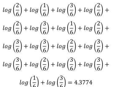
Considering the categorical data in Table 1. The x1 object is (A, E, M). The value frequency of x1

object is (2, 1, 3). The x2 object is (A, D, N). Its value

frequency is (2, 2, 3). The remaining objects have value frequencies of (2, 2, 3), (1, 2, 3), (3, 2, 3), (3, 2, 3), and (3, 1, 3). By using Definition 4, the entropy of Table 1 is

2 6 1 6 3 6 2 6 2 6 3 6 1 6 2 6 3 6 3 6 2 6 3 6 3 6 2 6 3 6 3 6 1 6 3 6 4.3774

By using the same mechanism, when x1 was taken

out from the table, the entropy becomes 3.8638. The

x1 object gives entropy different 0.5136.

Definition 5. Entropy of matrix of attribute value frequency

Suppose M is a matrix of attribute value

frequencies which is constructed from n categorical

data with m attributes, eij is the element of the ith row

and jth _{column of M. Since each data of M are}

independent, the entropy of M can be computed by

using

log , 0

By using Definition 5, the entropy of the categorical data in Table 1 is 4.3774. Suppose Table 2 is a new table obtained from Table 1 by taking out .

Table 2. Categorical dataset without .

U/A a b c

x2 A D N

x3 B G M

x4 C D N

x5 C G M

x6 C F N

A new matrix of attribute value frequencies (M1) can

be constructed from Table 2.

1 2 2 1 0 3 3 1 0 0 2 0

M1 has entropy 3.8638. By using

the above mechanism, the following matrices: M2,

M3, M4, M5, and M6 are the matrices of attribute

value frequencies of categorical data in Table 1

when object , , , and are

5678

1 1 3 1 1 2 3 1 0 0 2 0

2 2 2 0 1 3 3 1 0 0 1 0

2 1 3 1 1 2 2 1 0 0 2 0

2 2 2 1 1 3 2 1 0 0 1 0

2 2 3 1 1 2 2 0 0 0 2 0

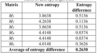
Table 3 shows the entropy difference of entropy of M1, M2, M3, M4, M5, and M6 to the entropy

of M. The average of the entropy difference is

0.2630.

Table 3. Entropy Difference

Matrix New entropy Entropy

difference

M1 3.8638 0.5136

M2 4.2638 0.1136

M3 3.8638 0.5136

M4 4.4148 0.0374

M5 4.4148 0.0374

M6 4.0148 0.3626

Average of entropy difference 0.2630

According to the AEVF method [12], the average of the entropy difference is called the maximum entropy gap. The outliers were x1, x3, and

x6. These objects have entropy difference greater

than the maximum entropy gap.

Definition 6. Weighted entropy of matrix of attribute value frequency

Suppose M is a matrix of attribute value

frequencies of categorical data DT=(U, A, V, f),eij is

the element of the ith _{row and j}th _{column of M, and}

W(x) is a positive continuous function. The weighted

entropy of matrix of attribute value frequency is

log , 0

Weighted Matrix Entropy Value Frequency (WMEVF) method improves the precision of AEVF method by implementing the weighted entropy of matrix of attribute value frequency. WMEVF method weighs the entries of attribute value frequency matrix by using weighting function. In this paper four weighting functions namely: range, variance, standard deviation, and square function are

used in experiment.

Matrix M7, M8, M9, and M10show the matrix

of attribute value frequency of the categorical data in Table 1 when range, variance, standard deviation, and square function are used.

1 2 0 0.5 1 0 1.5 1 0 0 2 0

2 6 0 1 3 0 3 3 0 0 6 0 2 3.4641 0

1 1.7321 0 3 1.7321 0 0 3.4641 0

4 4 9 1 1 9 9 1 0 0 4 0

The entropy are E(M7) = 3.4179, E(M8) = 2.4591,

E(M9) = 3.4091, and E(M10) = 4.3191. These values

are the total entropies. The remaining processes are the repetition of the former steps when an object is being taken out from the categorical data.

The following is the WMEVF algorithm with square function as the weighting function.

WMEVF with square function algorithm Input : Dataset – D (n objects, m attributes),

k target number of outlier

Output : k detected outliers

1. Read dataset D

2. Label all data objects as non-outliers 3. p = max(|Va|), Va= domain value, a = 1..m

4. Construct M, the p×m attribute value frequency

matrices. Fill all the entries with zero. 5. For each attribut ai, i = 1 to m do

Construct TF, the table of attribute value frequency which is sorted based on attribute value

Fill the ith _{column of M with TF, strating from}

the first row

6. Let the entropy total ET = 0 7. For each h, h = 1 to m do

For M(h), the hth _{column of M}

For each i, i = 1 to p do

If eih, the hth column and ith row of M and

eih ≠ 0

ET+= -2*( eih/n)2*log(eih/n)

8. SumE = 0

9. For each object xk, k = 1 to n do

M2 = M; Ek = 0;

For each attribute h, h= 1 to m do

Construct TF, the table of attribute value frequency of the hth _{attribute of the k}th

object

Subtracts TF from the hth _{column of M2}

5679 For each i, i = 1 to p do

If eih, the hth column and ith row of M2 and eih ≠ 0

Ek+= -2*(eih/(n-1))2*log(eih/(n-1))

SumE += ET - Ek 10. MaxEG = SumE/n

11. For each object xk, k = 1 to n do

If ET - Ek > MaxEG then kth object is an outlier

4. EXPERIMENTS 4.1. Experimental Setup

The experiment is done by using Intel Core i5 with 4 GB RAM. The algorithms were implemented in R programming language. The experiment used datasets from UCI Machine Learning repository, namely Mushroom, Nursery, and Adult [20]. The

Mushroom dataset contains 8124 instances with 23

attributes. The Nursery dataset contains 12960

instances with 9 attributes. The Adult dataset

contains 32561 instances with 15 attributes.

The Mushroom dataset is divided into two

groups, edible (4208 instances) and poisonous (3916 instances). The edible instances are assumed as the normal data. The poisonous instances are assumed as the outliers. The Nursery dataset is divided into

three groups: usual (4320 instances), pretentious (4320 instances), and great pretentious (4320 instances). The usual instances are assumed as the normal data. The pretentious instances are assumed as the outlier. The great pretentious instances can not be considered as the normal data nor the outlier. The great pretentious instances are not used in the experiment.

The first process in Adult dataset is omitting

the non-categorical data. Then, the Adult dataset is

divided into two groups: the persons who have income more than 50K (7841 instances) and the persons who have income less than or equal to 50K (24720 instances). The persons who have income less than 50K are assumed as the normal data, on the other hand, the persons who have more than 50K are assumed as the outlier.

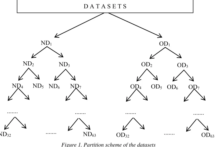
The formation of the experimental datasets is begun by partitioning the normal data and the outlier data as shown in Figure 1. Suppose ND1 and OD1 are the normal data and the outlier data. ND1 is partitioned into two same size partitions ND2 and ND3. ND2 is partitioned into ND4 and ND5. ND3 is partitioned into ND6 and ND7. The process is repeated until ND63. By using the same mechanism,

OD1 is partitioned into OD2, OD3, to OD63. The algorithm performance is observed by using two experiments namely the precision test and the complexity test. The experimental datasets for the precision test (PT) are formed by mixing each partition of the outlier (OD1, OD2, .., OD63) with ND1. The experimental datasets for complexity test (CT) are formed by mixing ND1 and OD1, ND2 and OD2, and soon. Table 4 shows the formation of the experimental datasets of the precision test. By using this mechanism, PTk will contain OD

outlier data.

Table 4.Dataset formation for precission test The experimental atasets for the

precision test (PT) PT1 OD1 + ND1 PT2 OD2 + ND1 PT3 OD3 + ND1 ... ... PT63 OD63 + ND1

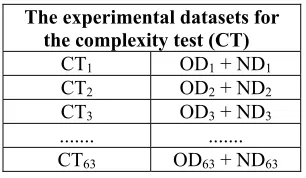
The experimental datasets for the complexity test (CT) are formed by mixing ND1 and OD1, ND2 and OD2, and soon. Table 5 shows the formation of the experimental datasets of complexity test. By using this mechanism, CTk will consist of

data. CTk is double in size comparing to CTk+1.

Table 5.Dataset formation for complexity test

The experimental datasets for the complexity test (CT)

CT1 OD1 + ND1

CT2 OD2 + ND2

CT3 OD3 + ND3

... ... CT63 OD63 + ND63

The precision test is done by observing the detected outlier from each experimental datasets for the precision test (PT1 .. PT63). Suppose, DOk is the detected outlier for PTk. The precision of the kth experiment is |_| |_|.

The complexity test is done by observing the time needed to detect outlier from each experimental dataset for complexity test (CT1 .. CT63).

4.2. Result and Discussions

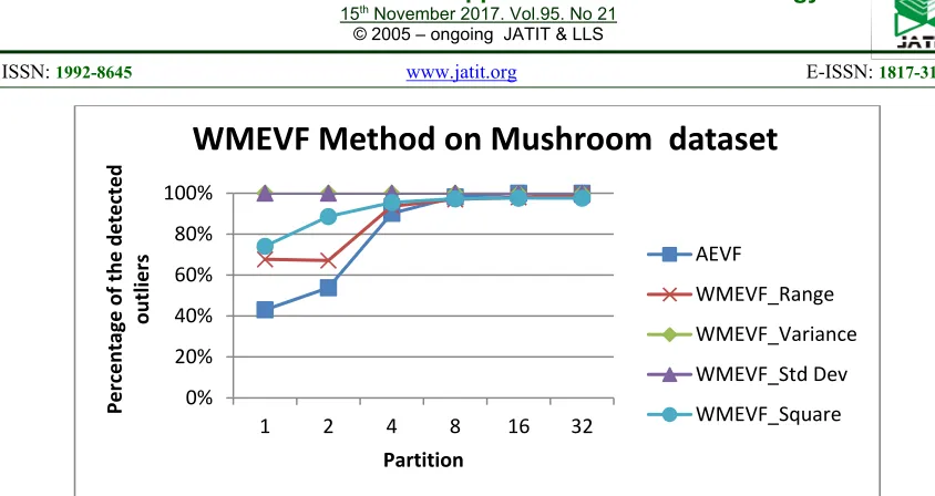
5680 square function are used in the experiment. Figure 2, Figure 3, and Figure 4 show the result of the experiments of the precision test. The performance improvements are shown in Table 6.

The square function is the only weighting function that improves the precision. The average precision improvement is 14% with standard deviation 7%. The square function does not decrease the precision for all datasets. Variance and standard deviation function give the highest precision improvement for Mushroom datasets but does not

improve the result for the Adult datasets. Range

function does not improve the performance AEVF. The performance of the weighting functions on the construction of WMEVF are same with the performance of the weighting functions on the construction of WAVF and WADOD [19].

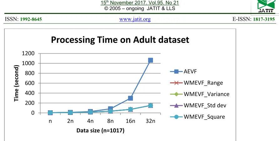
Figure 5 shows the time comparison between AEVF and WMEVF in detecting the outlier in Adult

dataset. Comparing to AEVF, WMEVF run faster than AEVF. AEVF method has complexity of

O(m*n2_{), while WMEVF has complexity of O(m*n).}

Comparing to AEVF, WMEVF has more efficient steps. In WMEVF, the recalculation is carried out by reconstructing the table of attribute value frequency of the data which is being taken out. Then, the table is subtracted from the attribute value frequency matrix. This matrix makes the WMEVF method runs faster then AEVF method.

5. CONCLUSIONSANDFUTUREWORKS

In this paper, a new outlier detection method called WMEVF has been proposed. It is built from AEVF by introducing matrix of attribute value frequency and weighting functions. Four weighting functions, namely range, variance, standard deviation, and square function are used to built WMEVF. Experiments of these new outlier detection methods

on Mushroom, Nursery, and Adult dataset show the

fact that :

1. The square function is the best weighting function in improving the performance of AEVF method.

2. By implementing the matrix of attribute value frequency, WMEVF reduces the algorithm complexity from O(m*n2_{) to}

O(m*n).

For the future work, the weighting function might be applied to improve the performance of outlier detection method for numerical or mixed type dataset.

REFERENCES

[1] Grubbs, F.E., 1969, Procedures for Detecting Outlying Observations in Samples,

Technometrics, Vol. 11, Issue 1.

[2] Hawkins, D.M., 1980, Identification of

Outliers, Chapman and Hall.

[3] Phyle, D., 1990, Data preparation for Data

Mining, Morgan Kaufmann.

[4] Chandola, V., Banerjee, A., and Kumar, V., 2009 Anomaly Detection: A Survey, ACM

Computing Surveys, Vol. 41, No 3, Article 15.

[5] Ajitha, P. and Chandra, E., 2015, A Survey On Outliers Detection In Distributed Data Mining For Big Data, Journal of Basic and Applied

Scentific Research, Vol. 5, Issue 2, page. 31- 38.

[6] Ilango, V., Subramanian, R., and Vasudevan, V., 2012, A Five Step Procedure for Outlier Analysis in Data Mining, European Journal of

Scientific Research, Vol. 75, No 3, pp.

327-339, EuroJournals Publishing, Inc.. [7] Gogoi, P., Bhattacharyya, D.K., Borah, B., and

Kalita, J.K., 2011, A Survey of Outlier Detection Methods in Network Anomaly Identification, The Computer Journal, Vol. 54,

No. 4.

[8] Koufakou, A., Ortiz, E.G., Georgiopoulos, M., Anagnostopoulos, G.C., and Reynolds, K.K. 2007, A Scalable and Efficient Outlier Strategy for Categorical Data, The 19th _IEEE

International Conference on Tools with

Artificial Intelligence.

[9] Arif, M. and Basalamah, S., 2012, Similarity- Dissimilarity Plot for High Dimensional Data of Different Attribute Types in Biomendical Datasets, International Journal of Innovative

Compting, Information, and Control, Vol. 8, No

2, pp. 1275-1297.

[10] Shih, M.Y. , Jheng, J.W., and lai, L.F., 2010, A Two-Step Method for Clustering Mixed Categorical and Numeric Data, Tamkang

Journal of Science and Engineeering, Vol. 13,

No. 1, pp. 11- 19.

[11] Zhao, X. , Liang, J., and Cao, F., 2014, A Simple and Effective Outlier Detection Algorithm for Categorical Data, Int. J. Mach.

Learn & Cyber, Vol. 5, pp. 469-477.

[12] Qamar, U., 2013, Automated Entropy Value Frequency (AEVF) Algorithm for Outlier Detection in Categorical Data, Recent Advances in Knowledge Engineering and Systems

Science.

[13] Grossman, J., Grossman, M., and Katz, R., 1980, The First Systems of Weighted

Differential and Integral Calculus, Archimedes

5681 [14] Salton and Buckley, 1988, Term Weighting

Approaches in Automatic Text Retrieval,

Information Processing and Management, Vol.

24, Issue 5, pp. 513-523.

[15] Gotoh, O., 1995, A Weighting System And Algorithm For Aligning Many Phylogenetically Related Sequences, Computer Applications in

The Biosciences (CABIOS), Vol. 11 no. 5, pp.

543-551.

[16] Getis, A. and Aldstadt, J., 2004, Constructing the Spatial Weights Matrix Using Local Statistic, Geographical Analysis, Vol. 36, Issue

2, pp. 90-104.

[17] Nakov, P., Popova, A., and Mateev, P., 2001, Weight Functions Impact on LSA Performance,

EuroConference: Recent Advances in NLP

(RANLP), Tzigov Chark, Bulgaria, 5-7

September 2001.

[18] Ustinovskiy, Y., Gusev, G., and Serdyukov, P., 2015, An Optimization Framework for Weighting Implicit Relevance Labels for Personalized Web Search, International World

Wide Web Conference Committee (IW3C2),

Florence, Italy, May 18-22, 2015.

[19] Rokhman, N., Subanar, and Winarko, E., 2016, Improving the performance of Outlier Detection Methods for Categorical Data by Using Weighting Function, Journal of Theoretical and

Applied Information Technology, Vol. 83, No 3.

[20] UCI Machine Learning Repository, https://archive.ics.uci.edu/ml/

[21] Koufakou, A., Secretan, J., Reeder, J., Cardona, K., and Georgiopoulos, M., 2008, Fast Parallel Outlier Detection for Categorical Datasets using MapReduce, IEEE International Joint

Conference on Neural Networks.

[22] Reddy, D.L.S., Babu, B.R., and Govardhan, A., 2013, Outlier Analysis of Categorical data using NAVF, Informatica Economica, Vol. 17,

No 1,pp. 5-13.

[23] Tan, S.C., Yip, S.H., and Rahman, A., 2013, One Pass Outlier Detection for Streaming Categorical Data, The 3rd _{International}

Workshop on Intelligent Data Analysis and

Management.

[24] Reddy, D.L.S. and Babu, B.R., 2013, Outlier Analysis of Categorical data using FuzzyAVF,

International Conference on Circuits, Power

and Computing Technologies (ICCPCT).

[26] He, Z., Xu, X., and Deng, S., 2005, An Optimization Model for Outlier Detection in Categorical Data, Proc. of 2005 International Conference on Intelligent Computing

5682

Figure 1. Partition scheme of the datasets

Figure 2. Precision comparasion of AEVF and WMEVF on Nursery datasets

0% 20% 40% 60% 80% 100%

1 2 4 8 16 32

Percentage 

o

f 

the 

detected 

outliers

Partition

WMEVF Method on Nursery Datasets

AEVF

WMEVF_Range

WMEVF_Std Dev

WMEVF_Variance

WMEVF_Square ND1

ND2 ND3

ND4 ND5 ND6 ND7

...

ND32 ... ND63

...

OD1

OD2 OD3

OD4 OD5 OD6 OD7

...

OD32 ... OD63

5683

Figure 3. Precision comparasion of AEVF and WMEVF on Mushroom datasets

Figure 4. Precision comparasion of AEVF and WMEVF on Adult datasets

Table 6. The Comparison of precision improvement by weighting function

Dataset

Average precision improvement Weighting function

Range Variance Standard deviation Square function

Nursery ‐16%  ‐1% ‐1% 9% 

Mushroom 6%  19% 19% 11% 

Adult 1%  ‐38% ‐38% 22% 

Average ‐3%  ‐7% ‐7% 14% 

Deviation std 12%  29% 29% 7% 

0% 20% 40% 60% 80% 100%

1 2 4 8 16 32

Percentage 

o

f 

the 

detected 

outliers

Partition

WMEVF Method on Mushroom dataset

AEVF

WMEVF_Range

WMEVF_Variance

WMEVF_Std Dev

WMEVF_Square

0% 20% 40% 60% 80% 100%

1 2 4 8 16 32

Percentage 

o

f 

the 

detected 

outliers

Partition

WMEVF Method on Adult Dataset

AEVF

WMEVF_Range

WMEVF_Variance

WMEVF_Std Dev

5684

Figure 5. Processing time of AEVF and WMEVF on Adult Dataset

0 200 400 600 800 1000 1200

n 2n 4n 8n 16n 32n

Time 

(second)

Data size (n=1017)

Processing Time on Adult dataset

AEVF

WMEVF_Range

WMEVF_Variance

WMEVF_Std dev