BIROn - Birkbeck Institutional Research Online
Pelliccia, Marco (2012) Risk-sharing and probabilistic network structure.
Working Paper. Birkbeck College, University of London, London, UK.
Downloaded from:
Usage Guidelines:
Please refer to usage guidelines at or alternatively
ISSN 1745-8587
Birkbeck Workin
g
Pa
p
ers in Economics & Finance
Department of Economics, Mathematics and Statistics
BWPEF 1214
Risk-sharing and probabilistic
network structure
Marco Pelliccia
Birkbeck, University of London
Risk-sharing and probabilistic network structure
Marco Pelliccia
∗Birkbeck, University of London
September 4, 2012
(PRELIMINARY AND INCOMPLETE)
Abstract
This paper studies the impact of a probabilistic risk-sharing network struc-ture on the optimal portfolio composition. We show that, even assuming identi-cal agents, we are able to dierentiate their optimal risk-choice once we assume the link-structure dening their relationship probabilistic. In particular, the nal agent's portfolio composition is function of his location in the network. If we assume positive asset-correlation coecients, the relative location of a player in the graph inuences his risk-behavior as much as those of his direct and undirect partners in a not-straightforward way. We analyze also two po-tential centrality measures able to select the key-player in the risk-sharing network. The ndings may help to select the central agent in a risk-sharing community and to forecast the risk-exposure of the players. Finally, this pa-per may explain natural dierences between identical rational agents'choices emerging in a probabilistic network setup.
JEL classication: D85, D81, O17.
Keywords: Informal insurance, Risk-sharing, Network.
1 Introduction
1992). Moreover, we also observe that the agents do not risk-share their endown-ments with all the individuals composing the main community1. Given these stylized
facts many authors have explained theoretically these ndings. The main challenge was to prove how mutual insurance relationships between peers could be stable in time despite the intuitive risk-sharing norm enforcement problem and the not-always perfect observability of individuals` endowments (monitoring problem). As Bloch et al. (2004) shows, there can be precise strategical reasons explaining partial-insurance schemes or the limited-size of the risk-sharing group given certain condi-tions. Specically, they suggest that if the links have double roles such as liquidity and information channel, we can expect just specic network structures arising as equilibrum of a strategical problem and guaranteeing the transfer-norm enforcement. Moreover, as Bramoullé and Kranton (2007) notices, individual optimal choices re-lated to the agent's link structure can lead to indirect negative externalities to the rest of the risk-sharing group and dierentiate the nal outcomes observed by the players. As Stack (1975), De Weerdt and University. United Nations (2002), Dercon and De Weerdt (2002), and Fafchamps and Gubert (2007) have empirically shown, the structure of the risk-sharing groups, in terms of connections between peers, seems far from being randomly formed. A common feature of all the studies about the risk-sharing problem that use a network analysis approach is to consider the transfers be-tween individuals passing through bilateral relationships (represented geometrically by a link between two nodes) so that, indirectly, the action of an agent can also inu-ence the one of another subject not directly connected with him. This intuitive and simple concepts have suggested the social scientists to investigate more the impact of the link-structure between risk-sharing individuals. Particular interest has been focused on the punishment schemes enforced by the nodes (through link rewiring strategies) to prevent deviations from the risk-sharing norm. In this paper we are not directly interested on studying the norm-enforcement problem but we focus the attention on the impact of a probabilistic link-structure on the agents` risk behavior, i.e. agents computing their optimal risk-exposure and connected in a risk-sharing structure through links consider the existance of the peers` connection not certain. The intuition comes from the fact that once the risk-sharing structure between peers is assumed probabilistic, the agents could nd optimal to modify their risk-exposure according to their location in the network. Facing a probabilistic link-structure, the impact of this uncertainty can be dierent between the agents whenever located in distinct locations through the network. There are many reasons to assume a probabilistic link-structure in a risk-sharing model using a network approach. The
1See for instance Townsend (1995), Udry (1995), Fafchamps and Lund (2003), Murgai et al.
existence of an agreement between two agents is usually explained by social or geo-graphic factors (family membership, friendship and geogeo-graphical proximity between many)2. However, these exogenous factors could change on time, being strongly
de-pendent on the exogenous agents`environment (the existance of a peer itself can be considered not perfectly certain in many cases). Moreover, if we reasonably assume that a link between two peers is a bilateral and strategical choice, changes on the ex-ogenous scenarios could let the peers reconsider their previous link-structure. In the interbank market for example we observe a nite number of institutions exchanging liquidity through short-period lending-contracts. This is a particular form of risk-sharing between institutions, foundamental for the diusion of liquidity in the bank-system. Each bank can bilaterally choose to open one or more liquidity channels as much as the relative partner-institutions. The protability of these connections can change with the arrival of a new information on the partners` risk or more generally with a change on the nancial environment. Being enforced by ocial contracts, the deviation from the risk-sharing norm is rarely observed in this case. However, the individual risk taken by the peers is not easily monitorable by the relative partners. This fact can lead to a classic moral hazard problem, in terms of risk-exposure or risk-strategies chosen by the institutions, not solvable by mechanisms of punishment studied using a network analysis approach (the perfect monitoring is a necessary condition to enforce a norm). On the other hand, the choice of a partner-institution seems to be strategical, function of specic market conditions (see for instance An-gelini et al. (1996), AnAn-gelini et al. (2009),Soramaki et al. (2007), Gabrieli (2011)). Given these facts, each agent may not consider the present bilateral relationships as xed but dynamic and function of dierent exogenous factors. In our model we argue that adding uncertainty at level of the link-structure can help to explain dierence on optimal risk-choices of identical agents belonging to a risk-sharing community and choosing their optimal portfolio composition. Thus, the probabilistic feature of the graph could help to underline the importance of an agent`s location analysis to understand relative advantages/disadvantages due to a player`s position.
in particular can also rene the literature on network analysis opened by Galeotti and Goyal (2010) and Bramoullé et al. (2010) between many. Finally, this paper can enrich the literature studying the impact of the network structure on the community`s risk-sharing degree (see for instance Ambrus et al. (2010), Battiston et al. (2009), and Stiglitz (2010)).
The paper is organized as follows. In the rst Section we present the main model where risk-sharing agents decide individually and optimally the composition of their portfolio between two assets, a risk-free and a risky one, assuming zero asset-correlation. In the second part of this section we study the impact on the optimal portfolio choices of a positive asset-correlation. We present in particular two examples of dierent network structures with specic structural features, underlining the importance of the relative nodes` location to explain the dierent risk-behaviors. In the last part of Section 2 we relax the perfect network observability assumption, assuming myopic nodes. Finally we discuss and test some node centrality measures and the implication of the model in terms of the minimizing-risk structure.
2 The model
In this section we introduce the model and the network notation. The model is composed by two main parts. In the rst one we study the nal equilibria assuming zero-correlation between the risky-assets, while in the second part we relax this assumption and produce two cases of study.
2.1 The network setup
We considerN agents linked each other according the adjacency matrixGn×n = [gij]
, where gij = 1 whenever the nodes i and j are connected by an undirected link
while gij = 0 otherwise. We assume also that gii = 0. We dene the degree of node i, di =
P
gij∀j ∈ N. For simplicity we will consider just connected components,
i.e. gij 6= 0 for at least one j ∈ N. Payos are described by Ui(x, δ, G) where δ ∈ (0,1) ≡ probability that if gij = 1 for some j at time t, gij = 0 at t+ 1. The
linklij between the nodesi and j describes the liquidity ow channel between these
two nodes. In particular without direct connection, two nodes can transfer liquidity each other just through a dierent path. We thus keep a generic denition for the link lij since it has not a precise physical meaning. Clearly lij exists if and only
if gij = 1. Finally, we dene a path as a non-empty graph P = (V, L) of the form V = {x0, x1, ..., xN} and L = {x0x1, x1x2, ..., xN−1xN}, where with xi∈N we dene
denition of structural symmetry using the notion of automorphism to describe two or more nodes symmetrically located in a graph. Formally an automorphism is a one-to-one mapping,τ, fromN toN of a graph G(N, L)such that <i, j >∈Lif
and only if <τ(i), τ(j)> ∈L. We can dene automorphism equivalence betweeni
andj ,i≡AE j, if there exists some mappingτ such thatτ(i) = j , and the mapping τ is an automorphism. Thus, if we nd such automorphism and we are interested
on studying the impact of the link-structure on the agents, we can analyze selected nodes of the graph representing the equivalence classes.
2.2 The zero-correlation case
There are n nodes/players, deciding how much invest of their unit capital on risky
asset, xi , and on risk-free asset, (1−xi) at timet. In particular, the risk-free asset
has variance σRF = 0, while the risky asset, σR > 0. Investing at t on the risk-free
asset yelds exactly the amount invested on it att+ 1, while the expected return from
the risky asset is positive and equal to pxih, where p is the probability of positive
return h. The identical agents are risk-averse and maximize their expected prot
choosing the optimal portfolio structure. At this stage the assets are identical for all the players but independent each other. The nodes are connected through a network structure describing the liquidity ow-path between the peers. We assume in fact that the agents transfer at each time t liquidity to each other following an
equal-sharing rule. Roughly speaking, at each t the agents agree to exchange liquidity
such that the nal income post-transfer is the same for all the agents belonging to the component. We assume also that the network structure is common knowledge and the players do not deviate from the sharing-rule. This means that the link lij
between two nodes i and j guarantees the respect of the risk-sharing norm, i.e., no
strategical deviation from the rule are allowed. As we will see formally, this setting and overall the common knowledge of the whole network structure guarantees the neutrality of the link-structure on the agents` optimal choices.
In absence of any connection (situation that we can dene as the autarky case), the expected income Y at timet for a generic agent i is
E[Yit] =xithp+ (1−xit)
for all i at time t . Consequently, the variance observed by playeri will be
V ar[Yit] =σR2x
2
it
assumption in particular gives us the possibility to exclude any other potential reason to observe heterogeneous choices between the players. The agents` instantaneous preferences are described by
uit(Cit) =E[Cit]−aV ar[Cit]
where a is the coecient of absolute risk-aversion and Cit is the consumption at
timet. Notice that if an agenti is not belonging to the risk-sharing group, Cit =Yit
. However, since we are considering just connected components (it does not exist a node such that the degree is equal to zero in our setting), each agent takes into account at eachtthe transfers to/from the rest of the players. Formally, the expected
income post-transfer is
Eit[Iit] = (xitph+ (1−xit))/n+ (ph
X
j6=i
xjt+ (1−xjt))/n (2.1)
and since we assume identical agents and no uncertainty on the network structure we expectxit =xjt for all iand j belonging to G. Thus, we can rewrite (2.1) as
Eit[Iit] =xitph+ (1−xit) (2.2)
or the expected income post-transfer is not changed. However, the variance ob-served by each identical agent at time t is
V ar[Iit] = (x2itσ
2
R)/n
2
+ (σR2/n2)X
j6=i
x2j = (x2itσ2R)/n (2.3)
so as expected the variance is function of the component size n. Thus, given the
expressions above, maximizing the utility function we can nd the optimal capital share x∗it invested on risky assets for all i,
x∗it =n(ph−1)/2aσ2R
The result is in line with the modern portfolio theory: The optimal capital-share invested on risky-assets is function of the returns of these assets, of their variance, of the risk-aversion coecient, and nally of the size of the risk-sharing group n.
To simplify the notation, from now on we dene the rate (ph−1)/2aσ2
R with k.
As anticipated in the introduction, next step will be to add uncertainty on the network structure assuming not certain the existence of each link att+ 1between
two generic nodes i and j such that gij = 1 at t. Formally, P rob[gij,t+1 = 1 |gij,t =
1] = (1−δ)∈(0,1)∀i, j ∈G. Notice that we do not allow the creation of new links
between the agents at this stage. As anticipated, this new model feature gives us the opportunity to describe the case where each agent cannot completely rely on the links he observes at time t. If this is the case, the location of each peer assumes a central
role for the optimal individual decision, i.e. we dierentiate the nodes` nal optimal choices. To give an example anticipating the formal results, let`s think about a star-shaped network structure. A central node is connected with many (symmetrically located) peripheral nodes so we can distinguish just two types of nodes. It is quite clear in this case that once we assume a probabilistic structure the position of the central node is more advantageous than that of the peripheral one. Firstly because the central node observes more direct partners (he can obtain liquidity att+ 1with
higher probability) and also because of the link`s channel feature he has got, i.e. a peripheral node can receive liquidity from another peripheral node if and only if the liquidity ow pass through the central node. As we will see formally, given the probabilistic feature of the graph, the most central node(s) will expect to risk-share with more agents than the peripheral ones. This advantage will dierentiate the players` nal choices.
Formally and for a generic network structure, the expected income post-transfer of a generic nodei now is
Eit[Iit] = (xitph+ (1−xit))/nit+ (ph)/nit
X
j6=i
θij,txjt +
X
j6=i
θij,t(1−xjt)/nit (2.4)
where nit ≡1/Eit[1n]3 and θij,t is the probability to observe the realization of the
partnerj. At this stage, we assume zero-correlation between the risky assets, so the
variance observed by each node at timet is
V ar[Iit] = (x2itσ
2
R)/n
2
it+ (σ
2
R/n
2
it)
X
θij,tx2jt (2.5)
Maximizing the utility function we nd the optimal x∗i at timet
x∗it =nit(ph−1)/2ασ2R (2.6)
We notice that the result is similar to the previous one except for the fact
that now the expected component size dierentiates the optimal nal agent`s choice. Intuitively a node i will observe the highest nit at time t than the rest of the nodes j if and only if his average distance with the rest of the agents (number of links to
reachj) is the smallest one. In the example of the star-shaped network structure, the
central node of the star will observe the highestnit and consequently he will be able
to choose the highestxitbetween all the nodes belonging to the component. However,
anticipating the further analysis, we can say that once we assume agents` sight bigger than one (a node i observes js distant more than one link from him), a simple
analysis of the nodes` degree is no more sucient to dene their centrality degree. In fact, even if in a star-network the centrality of the nodes is intuitively related to their degree, for a generic structure this is not always the case. In particular, at this stage, we can use our measurenit to characterize the agents/nodes` centrality scores.
The nodes` centrality scores are proportional tonit∀i∈G, i.e. the agents` centrality
is function of the expected number of partners with whom they will share their risk. Finally, notice that the individual peers` choices do not aect the single agent i`
decision at this stage. Without assuming dierent from zero-correlation between the risky-assets, the key feature dierentiating the agents is justnit . In the next section
we will relax this assumption and discuss the relative implications.
2.3 The positive-correlation case
In this section we assume positive correlation between the risky-assets. The correla-tion parameter is dened by ϕ∈ (0,1) . We still mantain the previous assumptions
and in particular the one dening the graph as probabilistic. Notice that the positive asset-correlation does not inuence the post-transfer expected income 2.4, but only the variance observed by the agents at each t. Formally,
V ar[Iit] = (x2itσ
2
R)/n
2
it+ (σ
2
R/n
2
it)
X
j6=i
θij,tx2jt + (2ϕσ
2
Rxit/n2it)
X
j6=i
θij,txjt (2.7)
Solving the optimization problem we can derive the best reply functions for each nodei∈G. In particular, we see that the optimal choice now is function also of the
partners` optimal ones,
x∗it=nit(ph−1)/2ασR2 −ϕ
X
θij,tx∗jt (2.8)
We notice that two main features aect now the nal optimal choice ofi. Firstly,
as we have seen in the previous section, the measures nit increases the optimal
the increasing optimal x∗jt of the peers negatively aects the agent i`s optimal
risk-exposure. Intuitively, higher is the risk taken by the peers, higher is the risk observed by each node, given the positive asset-correlation. However, the j partners`optimal
choices are discounted by their distance with the node i: The i`s location aects
again his optimal choice but in a reverse way. This is possible since the risk taken by the i‘s peers, given ϕ∈(0,1), is assumed partially substitute of the risk taken by
i himself. However, similarly to the discount coecient used by Bonacich (1987) in
his centrality measure, the choices of thei‘s partners are discounted byθij , function
of the distance from i to j nodes. Summarizing, the nal optimal choice is function
of nit , that depends on the relative location of i at time t in the network and on
link probability δ, of the correlation coecient ϕ, and nally of the peers` optimal
choices, function themselves of their relative locations.
To underline the importance of a structural analysis to forecast the optimal agents` behaviors, we present below two examples considering dierent starting net-work structures. As anticipated we have chosen two specic graphs such that we can easily observe the impact of dierent locations on the nal nodes` choices. The rst example considers three nodes connected through a line-shaped link-structure (see Figure 2.1). The second one describes a seven-nodes network in which two symmet-ric nodes have the highest degree and are respectively connected to two symmetsymmet-ric pairs of peripheral nodes, and nally one node, located as a bridge between the two automorphic subgraphs.
Figure 2.1: 3 nodes Star
In this rst example we start with a 3 nodes line-shaped network structure, where the node labelled 2connects 1 and 3. We can just study the nodes` choices of 1and 2 since 3 belongs to the same equivalence class of 1. Assuming k = 0.2 and for the
moment ϕ= 0 we nd the following optimal x∗it (vertical axis) for δ between 0 and
Figure 2.2: 3 nodes Star with zero asset-correlation. We notice the advantage of the node 2 over 1 and 3 for all theδ ∈(0,1).
As we can see, the node 2 mantains an advantage over 1 and 3 for all the
values of δ between 0 and 1. Before analyzing the second structure, we study the
eect of dierent positive values ofϕ on the optimal risky choice. To do this, we x
arbitrary values of δ, (0.3,0.5,0.7,0.8), and compute the optimal x∗it for dierent ϕ
values (horizontal axis).
Figure 2.3: 3 nodes Star with positive asset-correlation and δ = 0.3. The node 2
chooses optimal x higher than 1 and 3 nodes for allϕ∈(0,1).
In the Fig.2.3 above the link probability is setted toδ = 0.3and related expected
component-size vectorn¯= (2.19,2.4,2.19) . We observe that the node 2 still has an
advantage respect to 1 and 3. The probabilistic graph feature simply decreases the optimal agents` choices without reverting the node 2`s advantage over 1 and 3. This is possible since, given this specic structure, the node 2 has both an advantage in terms of higher nit and relative location of his partners. As we will see in the next
[image:12.612.190.420.384.534.2]present the optimal choices forδ = 0.5 ,
Figure 2.4: 3 nodes Star with positive asset-correlation and δ= 0.5.
As we can see the results do not change qualitatively from the previous one. The node 2 mantains an higher advantage over 1 and 3 than in the previous case. Following, we present other two for δ= 0.7and 0.8 respectively.
[image:13.612.103.273.348.449.2]Figure 2.5: 3 nodes Star with positive asset-correlation and δ= 0.7.
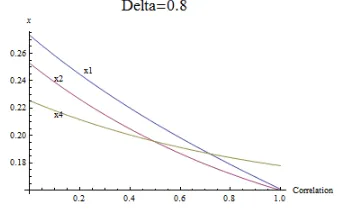
Figure 2.6: 3 nodes Star with positive asset-correlation andδ = 0.8. Forϕ >
0.7 we start to see the previous node
2`s advantage reverted in favour of the peripheral nodes.
Summarizing, increasing the probability δ, given this star-shaped structure, we
observe a general decreasing of the nodes` optimal risk-exposure but also a decreasing (in favour of the peripheral nodes after certain values ofδ) of the relative dierences
onx∗it between the players.
[image:13.612.338.508.349.444.2]classes composing the graph, thus we will analyze just the optimal choices of the representative nodes 1,2 and 4 of their respective equivalence classes.
Figure 2.7: 7 nodes structure
We start again analyzing the zero-correlation case. The optimalx∗it forδbetween
0 and 1 are described below,
Figure 2.8: 7 nodes structure with zero asset-correlation. Until around ϕ= 0.1 the
node 2 has the highest optimalx. The peripheral nodes choose the lowest optimalx
for all ϕ∈(0,1).
It is interesting to notice that until a particular level of δ, the most central node
is the node 2 (and consequently we expect 2 to choose the highest capital-share on risky assets), but after that, the nodes 1 and 3 appears to have the highestnitscores.
This rst picture helps us to underline the impact ofnit, function of the i`s location,
and of δ, on the nal optimal choice. As we have done previously, let`s assume now
[image:14.612.188.419.317.480.2]Figure 2.9: 7 nodes structure with positive asset-correlation. The node1
chooses the highest x. The peripheral
nodes choose the lowest optimalx for
[image:15.612.339.508.61.158.2]allϕ∈(0,1).
Figure 2.10: 7 nodes structure with positive asset-correlation. We can no-tice the decreasing dierences between the optimal x of the nodes 2 and 4,
once we increase the asset-correlation.
It is interesting to observe in the Figure 2.9 that the dierences on the optimal choices of the nodes2 and the peripheral ones become smaller increasing the
asset-correlation. This is due to the smaller degree dierence between them and also to the negative eect given by the relatively advantageous location of the nodes1and 3. The nodes 1 and 3 observe with higher probability the peripheral nodes (with
lownit scores) while the node 2 observes 1 and 3 as direct partners. This dierence
explains in part their relative advantage. In the Figure 2.10 we can observe more clearly the impact of the asset-correlation on the nodes` location. For δ ≥ 0.7 we
notice the advantage of the peripheral node 4 over 2 for ϕ > 0.5 . The intuition
behind is that when the structure is particularly uncertain and the asset-correlation relatively high being more connected or at a shortest distance with other peers is not more advantageous.
Following we present the optimal x∗it for δ= 0.7 and 0.8respectively,
Figure 2.11: 7 nodes structure with positive asset-correlation andδ = 0.7.
Figure 2.12: 7 nodes structure with positive asset-correlation and δ= 0.8.
In the next section and before discussing about potential structural measures, we discuss in more details the centrality measure nit. As anticipated in the
[image:15.612.338.507.508.613.2] [image:15.612.105.273.513.615.2]2.4 The centrality measure
n
itWe have seen from (8) how the agents` nal optimal choices are dependent of their relative location in the network. Moreover, the link between two peers aects in opposite ways the risk taken by them. As we have previously remarked, the positive impact is described by thenit score, while the negative one is catched by the node`s
partners choices and the positive asset-correlation coecient. To compute nit we
calculate the expected number of peers with whom the agenti is expecting to share
his risk. This centrality measure in particular is function of the average distance between the nodes: More links a nodeineeds to walk through to reach their partners js, lower probability he faces to reach them, assuming δ i.i.d.. Formally,
nit=
1
Pn
m=1pm(Hm)m1
(2.9)
where m is the number of peers risk-sharing including i, δ is the probability
dened between 0 and 1 that an existing link at t will exist at t+ 1, and pm(Hm)
denes the probability to observe the subgraph Hm generated by a specic set of
ties (connecting the node i to other m −1 nodes) containing m nodes including i. Notice that we can have more than one combination of paths containing i and
m−1 other nodes. The nit measure, dierently from the Bonacich one, takes into
account all the paths including i and not only the ones emanated from this. The
density of the graph and consequently the average distance between the nodes aects directly the measurenit. A more dense graph in fact leads to higher number
of subgraphs Hm (increasing the number of combinations of m nodes including i
). However, nit is also function of the link-probability δ, so as we have seen from
the examples presented above, it is not always the case that for all the values of
δ ∈ (0,1) the node with lower average distance from the rest of the agents has the
highest nit score. Summarizing, the nit centrality measure takes into account all
the possible paths passing through the node i at time t, it allows for owing by
parallel duplication, and nally it works on connected graphs (the distance between two nodes belonging to two dierent unconnected component is assumed innite). In this model we assume also independent probability over the existance of each distinct path. Finally we want to stress out the fact that this measure counts the expected number of peers a nodeiis attached to at timet.This means that dierently
from the mainstream of the network centrality measures,nit is node-founded even
if the paths to reach each peer directly inuence the measure. We can observe a clear example of this ambiguity in the second network structure presented above. In that case, the node with highest closeness and betweeness scores is the node 2,
we nd that just for particularly low link-probability δ the node 2 has the highest
score. Intuitively, even if the node can reach in less steps the rest of the peers, with higher probability than 1 and 3 he can nd himself in isolation. Following
the Sabidussi (1966) criteria qualifying a centrality measure, we can notice that nit
fully satisfying them. In particular, adding a tie to a node i increases his nit score,
and adding a tie anywhere in the network never decreases his centrality. However, as Borgatti and Everett (2006) underlines, these criteria do not fully explain the centrality of a node. This feature can be also observed in our model: The total-centrality of an agent is the result of two total-centrality measures as we can see from the agent's best reply function. Thus, the nit measure in our model describes the
geodesic relative advantage/diadvantage of a node without giving us any information about the relative advantage/disadvantage of the inuence of a node. We have to remark that the nit measure is directly connected to the Katz (1953) measure and
consequently to theBonacich (1987)'s one. Their measures are weighted counts of the number of walks originating (or terminating) at a given node. This means roughly speaking that long walks count less than short ones. However, the nit measure, as
previously said, counts the expected number of nodes reached by weighted paths (not necessarely edge or vertex-independent).
We show below, as example, how we can compute the nit measure for the specic
case of a star-shaped network structure with one central star-node and n peripheral
nodes,
nit=
1
Pn
c=1 1
c
(n−1)!
(c−1)![(n−1)−(c−1)]!(1−δ)c
−1δn−c
njt =
1
δ+Pn
c=2 1
c
(n−2)!
(c−1)![(n−2)−(c−1)]!(1−δ)
c−1δn−c
with i labeling the star node and j the peripheral one.
2.5 Myopic nodes and positive asset-correlation
In this section we relax the perfect knowledge of the network structure assumption, assuming that the agents can observe just their direct neighbors (nodes 1-link distant) and neighbors 2-link distant. We mantain the rest of the previous assumptions as much as the positive asset-correlation one. We start presenting the 7-nodes structure previously studied, assuming 1-link nodes` sight and following, the case for 2-links nodes` sight. Notice that for the particular1-link nodes` sight assumption, nit varies
between 1 and dit , the degree of node i. Assuming δ = 0.3 we obtain the following
Figure 2.13: 7 nodes structure, positive asset-correlation, myopic nodes (1 link sight) and δ= 0.3.
We can clearly see the negative eect of being connected to the nodes {1,3} faced by the rest of the nodes, for low correlation values (ϕ < 0.7 ). However, we observe
the reverse situation for correlation values above 0.7: The nodes {2,4,5,6,7}choose higher x∗ than 1 and 3, and in particular the node 2 has highest x∗. Notice that
assuming 1-link sight the nodes 1 and 3 observe highest number of partners for all the values of δ between 0 and 1. However, the peer eect is particularly clear for
the node 2 choosing lower x∗it than the peripheral nodes for some asset-correlation
level (the same is true for valuesϕ >0.7comparing the nodes {1,3} with {4,5,6,7}).
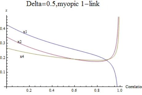
Forδ = 0.5 we obtain,
Figure 2.14: 7 nodes structure, positive asset-correlation, myopic nodes (1 link sight) and δ= 0.5.
We notice immediately that for δ ≥ 0.5 we don`t have the particular result
ob-tained in the previous picture forϕ > 0.7. However, even in this case we observe the
peer eect reverting the relative advantage of the node 2 on {4,5,6,7} for ϕ >0.9.
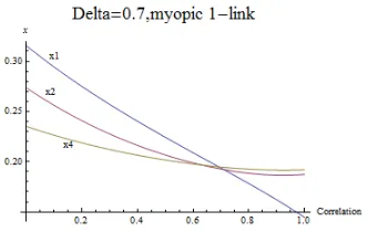
[image:18.612.189.420.430.585.2]Figure 2.15: 7 nodes structure, posi-tive asset-correlation, myopic nodes (1 link sight) and δ= 0.7.
Figure 2.16: 7 nodes structure, posi-tive asset-correlation, myopic nodes (1 link sight) and δ = 0.8.
At this highδ levels, we observe the reverting advantage noticed before for lower
asset-correlation coecients.
Now, as anticipated, we generate the results assuming 2-links distance sight. This case appears to be more interesting than the previous one since the node 2 is the only player able to see the whole structure, i.e. the strategical location of this agent has a strong impact on the nal optimal agents`choices. For δ= 0.3 we obtain
Figure 2.17: 7 nodes structure, positive asset-correlation, myopic nodes (2 link sight) and δ= 0.3.
At this probability level the node 2 observes highestnitthan the rest of the nodes.
The node 2 mantains an advantage for all the ϕ values. Even in this case the peer
[image:19.612.189.421.361.505.2]Figure 2.18: 7 nodes structure, posi-tive asset-correlation, myopic nodes (2 link sight) and δ= 0.5.
Figure 2.19: 7 nodes structure, posi-tive asset-correlation, myopic nodes (2 link sight) and δ = 0.7.
Figure 2.20: 7 nodes structure, positive asset-correlation, myopic nodes (2 link sight) and δ= 0.8.
The results are qualitatively dierent forδ >0.3: The peer-eect becomes central
to understand the choices` dierences. In this case, the nodes 1 and 3 have a slightly highernit score than the node 2but, for the fact that they are attached to relatively
disadvataged located nodes, the dierence with node 2'optimal choice is amplied. Notice that if we were studying the centrality a la Bonacich it would be not sucient to understand the results obtained above. This is due to two main features of the model. Firstly, the fact that the results depend mainly on the two parameters δ
and ϕ. Secondly, the fact that the link in our model is channel of two dierent
things. It represents both the liquidity channel between the agents and also a canal through which the peers` risk is spread through the network. The models using the β centrality measure or generally the eigenvectors centralities assume that the
peers`choices impact on an individual decision is either positive or negative. In this model, both positive and negative eects are present at the same time, as we can see from the 2.6. Having higher nit means for a generic node i to face higher
risk-pooling opportunities, while higher Bonacich centrality scores of the direct partners increase the risk observed by i for positive correlation coecients ϕ. We can also
2.6 Structural analysis
[image:21.612.188.426.503.644.2]In this section we try to underline the impact of the starting network structure on the nal optimal agents` choices. Before starting the proper analysis it is necessary to clarify the meaning of the link between the agents as much as the results obtained so far. What we can understand from 2.6 is that the connection between two nodes is both a channel of liquidity and a way to receive the peers` correlated risk. This double feature represents the central key of the model. Analyzing the literature on risk-sharing using a network analysis approach we see that the negative impact of the peers was usually represented by their risk of default and its related consequences. This implies that with this setting the link between two agents could exist if and only if there has been a previous liquidity ow between the interested parts. In this model is not necessarely the case. The connection represents the existance of a risk-sharing norm between two agents and no previous liquidity exchange is necessary to observe a connection between two nodes. This dierence becomes central to explain the agents` behaviours observed in our model, overall if we recall the assumption of no-deviation from the risk-sharing norm on the agents` strategies. In addition, the double link`s feature prevents us to use only the Bonacich centrality measures to understand the agent` choices. In fact, as underlined before, the Bonacich centrality scores, a volume measure using the Borgatti 2006 terminology, could just explain the negative\positive impact of the peer risk-choices but fails to take into account at the same time the two opposite directions. Specically, the Bonacich measures can help us if and only if we assume one specic direction of the peers` impact on the agent`s nal decision; In particular, the inuence of a node's choice on the peers' ones. Looking to the following picture we notice this feature,
Figure 2.21: Bonacich centrality for the 7 nodes structure.
According to the Bonacich centrality scores, for δ values between 0 and | 0.5 |
relative advantage given by the location of the nodes1and3, but we miss the negative
eect given by the same location once we assume in the model the ow of a positive correlated risk. We notice that the node 2 for example is particularly negatively
aected by the close connections with the nodes 1 and 3, respectively linked to two
peripheral nodes (located in the worst geodesic position). However, as we can see from the b.r.f. above, for particularly high correlation coecients, and uncertainty on the ties' future existance, the peripheral nodes are those in advantageous location. Given the dual-feature of the link we suggest two dierent tools, focusing each on one of the two link mentioned characteristics: The F¯- and the
Intercentrality-measure. The rst one measures the fragmentation of the network due to the elim-ination of a node i. In particular, the proposed F¯-measure is a modied version of
the F-measure explained by Everett and Borgatti (2010) and takes into account the
expected size of the components created after the elimination of i from the main
connected component. This measure in particular can help us to understand the impact of the elimination of a specic agent on thenit centrality measure. Formally,
¯
Fit= 1−
P
j6=injt(njt−1) n2(n−1)
bounded above at 1. This measure catches an important feature of network
structure. Intuitively, F¯ explains the impact of a node i on the risk-sharing group
in terms of his structural centrality. As example consider a star-shaped structure with the nodei as central agent connecting the rest ofn−1js nodes through single
links with them. The elimination of the node i from the component fragments the
whole structure and creates n−1 single-node components. In terms of F¯it score,
we will obtain F¯it = 1, its maximum level. Moreover, F¯it = 1 means that x∗ jt = k,
their optimalxwhen they do not risk-share with other peers (autarky case). On the
other hand, suppose the case of a starting graph where the elimination of a node i
leaves a component of n−1nodes perfectly connected (the resulting component is
a connected network where all the j nodes can reach each other with a direct link).
In this case, the impact of i-elimination will be relatively the smallest (the exact
¯
Fit score depends also on the δ chosen) since the rest of the j nodes can still enjoy
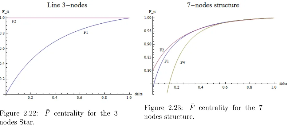
the risk-pooling eect in the most eective way. The F¯ scores for the 3-nodes and
7-nodes structures presented above for δ∈(0,1)are the following,
forδ6= 0.5since the inverse of the norm of the largest eigenvalue of the adjacency matrix Gis0.5. Moreover, we added the negative sign in front ofδ since we want to analyze the centrality in the
Figure 2.22: F¯ centrality for the 3
[image:23.612.93.560.56.261.2]nodes Star.
Figure 2.23: F¯ centrality for the 7
nodes structure.
We can see that for the 3-nodes structure the node with the highest F¯ score is
the node 2 for all the δ ∈ (0,1) and equal to 1: Taking out this node leads to the
maximal damage to the structure, leaving the nodes 1 and 3 isolated. For the 7-nodes structure, again the node 2 has the highestF¯ score, but as we can see from the
picture above hisF¯ centrality, for δ higher than 0.5, starts to be closer to the node 1
and 4`s ones. We will produce now the results for theF¯ scores of the myopic nodes
[image:23.612.91.550.429.648.2](observing just their direct neighbors or 1-link distant neighbors and 2-link distant neighbors) composing the 7-nodes structure,
Figure 2.24: F¯ centrality for the 7
nodes structure with myopic nodes (1 link sight).
Figure 2.25: F¯ centrality for the 7
nodes structure with myopic nodes (2 links sight).
In the rst case we notice that the node 1 (and symmetrically the node 3) has the highestF¯ score, i.e. the elimination of this node damages more the risk-sharing
elimination and not multiple-nodes one. Assuming 2-links distant sight, the nodes 1 and 3 remain the most central according to theF¯ measure.
The second measure is a particular centrality tool developed by Ballester et al. (2006) that helps us to understand the impact of a nodeion the Bonacich centrality
scores of his peers. In particular this measure can tell us the negative impact of the relative peer location. Formally,
cit(g, β) = b(g, β)−b(g−i, β) + 1
or alternatively,
cit(g, β) = bit(g, β) +
X
j6=i
[bjt(g, β)−bjt(g−i, β)]
withbit(g, δ)dening the Bonacich score of the nodeibelonging to the component g at time t. Computing the intercentrality scores for our 7-nodes structure, we nd
[image:24.612.212.404.352.414.2]the following results for |δ|∈(0,1),
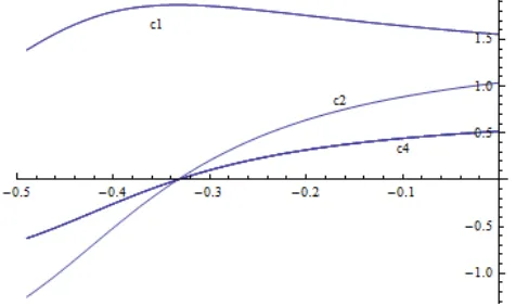
Figure 2.26: Intercentrality scores for the 7 nodes structure.
As we can see from the table, when we assume relatively smallβ coecients, the
higher impact is given by the elimination of the nodes 1 and 3. Once we assume
higherβ, the central node is the agent 2.
Summarizing, the parallel analysis of these two measures could explain the impact of each nodeiin terms of thei`s role in the network. HighF¯i values tell us that the
cohesion of the network strongly depends on the node i, while ci(g, β) scores show
the i‘s peer eect on the other nodes. The net impact on the nal agents` choices
will depend on the parametersδ and ϕassumed.
[...]
Talking about the structure impact on the agents` choices we focus the attention now on the average agent`s distance from the rest of the group. The average distance measuredit for a node i at time t gives us the geographical information about an
agent`s location in the network. Formally,
dit=
P
Again, smallerditdoes not necessarely mean to choose higherx∗it, as we have seen
in the previous examples. However, we argue that, under certain conditions, there exists just a unique structure minimizing the risk taken by the agents, and this is the line structure.
We start proving that starting from a line-shaped network structure, any rewiring leads to higher average distance between the nodes.
Claim 1. Any structure dierent from the line-shaped one leads to higher average distance between the nodes.
Proof. Assume a starting line-shaped network structure of n ≥ 4 nodes as in the
Figure (2.27). Let`s label the nodes asj1, j2, ..., jn, where with the node indexed with
1 we label one of the two peripheral nodes (the other one consequently is indexed with n ). For simplicity (but without aecting the nal conclusion) we modify the
structure, cutting the link between the rst node of the line,j1, with the second one,
j2 , and we activate a new link betweenj1 and a generic nodejm , withm ∈[3, n−1]
as in the Figure (2.28). In this way, the structure now is not more a line but a generic tree with the same number of links between the nodes. Firstly, notice that for the node 1, linking with another node dierent from j2 can only be benecial in terms
of average distance with the rest of the nodes, i.e. the net-impact for this node will be positive. The same we can say about the nodesjm+a with a∈[0, n−m]. In fact,
for all of them it is changed the distance (now shorter) from the node j1 without
aecting the distance with the rest of the nodes. Thus, until now we can say that
j1 and jm+a will have a positive net-impact from the new link-rewiring. Now, let`s
divide the rest of the nodes, indexed as jh, with h ∈ [2, m−1], in two sets: One
composed by nodes such that m −h ≤ h −2 , or h ≥ m+2
2 , and one such that
h < m2+2 . Notice that doing this we are dividing the jh nodes between those nodes
such that the distance between them andjm node is smaller/equal than the previous
distance (before the rewiring) withj1 ,with the ones where the converse is true. The
intuition behind that comes from the fact that for the nodes such that h≥ m+2
2 , we
expect a positive net impact from the rewiring since they will be linked to the node
j1 in shorter distance, while for the other ones, the new structure will connect them
toj1 with a longer path than before the rewiring. Finally, we need to show that the
number of nodes belonging to the latter group is always lower than the number of the rest of the nodes belonging to the network, for any line-shaped structure of n
nodes. In particular, it must be true that m+2
2 −1≤1 +n−
m+2
2 orm+ 2≤n+ 2.
This is always true with strict inequality, given our initial assumptions on m and n.
Figure 2.27: Seven nodes Line. Figure 2.28: Seven nodes Line rewired.
Given this result we can show that, under certain conditions, the line-shaped network structure is the one minimizing the total risk taken by the agents belonging to the component.
Claim 2. Given our assumptions and ϕ such that ∂xi
∂dit < 0, the net-work structure minimizing the total risk taken by the agents is unique and it is the line-structure.
Let`s underline the fact that the total risk (variance) observed at each t, is function
of the capital shares invested by the agents on the risky-assets. We have previously showed that the optimalx∗it chosen by a generic agent iis a function f(nit)and that nit is a function g(δ) of the probability δ ∈ (0,1). Moreover, nit depends on the
relative location of the nodeiat time t. In fact, as we can see from the formula used
to computenit, shorter average distancedit implies higher probability (in average) to
observe the partner nodes and consequently highernitscore. In particular, let`s dene
withlG = n(n1−1)
P
ditthe total average distance between the nodes of the component
G. As we have said, ∂ni
∂di <0since more a nodeiis distant from the rest of the nodes (more links betweeniand anyj ∈G) lower is the expected number of agents observed
att+ 1 (lower nit). Thus, by chain rule we have ∂x∗
it
∂dit =
∂f(.)
∂nit
∂g(.)
∂dit −ϕ
P
j6=i ∂θij
∂dit
∂x∗jt
∂dit , with ∂θij
∂dit < 0 for the same reason explained for nit, and not clear sign of
∂x∗jt ∂dit since it depends on the impact of the change of average distance ofi, dit , on the average
distancedjt, i.e. ∂x∗
jt
∂dit =
∂x∗
jt
∂djt
∂djt
∂dit . Thus, the net impact of an increasing ofdit on the optimali`s choice depends also onϕand on ∂x
∗
jt
∂dit. Underlined this fact and given the previous claim on the structure maximizing the distance between the nodes, we can say that, given a specic value of ϕ small enough or such that P
j6=i ∂x∗jt
∂dit < 0, the network structure with highest average distance between the nodes is the line, and this will be also the structure with lowest individual risk taken by the agents.
We generate an example that shows precisely what we have claimed. In the pictures below we present two graphs composed by 4 nodes: A star-shaped and a
line-shaped one. As we can see from the b.r.f. below, givenδwe are able to compute
theϕsuch that the line (higher average distance) guarantees to a specic node higher
Figure 2.29: 4 nodes Star. Figure 2.30: 4 nodes Line.
Notice that the previous claim is only valid for ϕand δ such that ∂xit
∂dit <0. This restriction is necessary since forϕandδ such that ∂xit
∂dit >0the correlation coecient is high enough to revert the positive eect on the optimalxitof an higher nit score to
[image:27.612.104.271.338.447.2]a negative one. Intuitively, for high enough asset-correlation levels, being connected with more nodes (in expected value) and overall linked with nodes in advantageous locations could become not-benecial for some agent (see the Figures below).
Figure 2.31: 3 node`s best reply for
ϕ ∈ (0,1) belonging to the Star or
[image:27.612.340.507.343.442.2]the Line (as peripheral node) forδ= 0.3.
Figure 2.32: 3 node`s best reply for
ϕ ∈ (0,1) belonging to the Star or
[image:27.612.328.511.364.618.2]the Line (as peripheral node) forδ = 0.5.
Figure 2.33: 3 node`s best reply for
ϕ ∈ (0,1) belonging to the Star or
the Line (as peripheral node) forδ= 0.7.
Figure 2.34: 3 node`s best reply for
ϕ ∈ (0,1) belonging to the Star or
the Line (as peripheral node) forδ = 0.8.
Without reporting the plots, we remark that for the nodes 1 and 2, we nd that
is possible since intuitively these nodes benet from the star structure in terms of both shorter average distance and peer eect.
Notice that the model does not take into account the leverage between the agents and the default of a peer is not allowed in this model. Even if we assume that the link-structure is probabilistic, the consequence of an exit from the risk-sharing group of a node does not aect directly the income of the other peers. This is possible since we are considering a two-periods game with no repayment-problem. For the same reason, we do not study in this model contagion eects or related problematics usually underlined in the literature.
[ADD THE CASE FOR THE 3 NODES NET]
3 Conclusions
In this paper we show that, assuming a probabilistic network structure between risk-sharing agents, deciding their optimal capital share to invest on risky assets, we are able to dierentiate the agents`optimal choices, without assuming any dierence on agents'degree of risk aversion. In particular, the nal optimal choices will be function of their relative location through the network. We analyxe also two measures able to characterize the most central agents in our model: One is a modied version of the F measures proposed byEverett and Borgatti (2010),F¯, and the other one, the
Intercentrality measure discussed in Ballester et al. (2006). In particular, we nd that theF¯ measure can be useful to pick up the key-player, or the most inuencial
representing the existance of a risk-sharing norm between peers, is often explained by previous social-relationships between the partners. However, monitoring constraints and exogenous changes on the social-connections can undermine the existance of the liquidity channels between the parts, i.e. precautionary risk-behaviors could be the optimal startegy in such environment.
The aim of this paper is to improve the risk-sharing literature using a network analysis approach. The previous works studying the structure of the bilateral rela-tionships between agents have focused the attention mainly on the dynamic of the network and in particular on the potential norm-enforcement using links-rewiring as deviation punishment strategy. This paper underlines more the importance of the structure on the optimal risk-choice taken by the connected agents. Further extesions could rene the probabilistic setting, linking the link-probability to the risk-exposures of the agents for example. Doing this way one of the central factors that in this model was assumed exogenous could be endogenized through the players` optimization problem. Moreover, adding the dynamic on the link structure can com-plete the model opening new questions in terms of expected equilibrium structures and thus explain the dynamic of the network structure observed in the interbank market between many. Given the probabilistic feature of the risk-sharing network and given specic asset-correlation coecients for example, it could be interesting to study optimal link-rewiring strategies and related equilibrium structures.
References
Ambrus, A., Mobius, M., and Szeidl, A. (2010). Consumption risk-sharing in social networks. Technical report, National Bureau of Economic Research.
Angelini, P., Maresca, G., and Russo, D. (1996). Systemic risk in the netting system. Journal of Banking & Finance, 20(5):853868.
Angelini, P., Nobili, A., and Picillo, M. (2009). The interbank market after August 2007: what has changed and why? Banca d'Italia.
Ballester, C., Calvó-Armengol, A., and Zenou, Y. (2006). Who's who in networks. wanted: the key player. Econometrica, 74(5):14031417.
Bloch, F., Genicot, G., and Ray, D. (2004). Social networks and informal insurance. Technical report, mimeo graph.
Bonacich, P. (1987). Power and centrality: A family of measures. American journal of sociology, pages 11701182.
Borgatti, S. and Everett, M. (2006). A graph-theoretic perspective on centrality. Social networks, 28(4):466484.
Bramoullé, Y. and Kranton, R. (2007). Risk-sharing networks. Journal of Economic Behavior & Organization, 64(3-4):275294.
Bramoullé, Y., Kranton, R., and DkAmours, M. (2010). Strategic interaction and networks.
De Weerdt, J. and University. United Nations, W. I. (2002). Risk-sharing and en-dogenous network formation. WIDER DISCUSSION PAPER WDP.
Dercon, S. and De Weerdt, J. (2002). Risk-sharing networks and insurance against illness. Centre for the Study of African Economies, Working Paper Series, 17.
Everett, M. and Borgatti, S. (2010). Induced, endogenous and exogenous centrality. Social Networks, 32(4):339344.
Fafchamps, M. and Gubert, F. (2007). The formation of risk sharing networks. Journal of Development Economics, 83(2):326350.
Fafchamps, M. and Lund, S. (2003). Risk-sharing networks in rural philippines. Journal of development Economics, 71(2):261287.
Gabrieli, S. (2011). The microstructure of the money market before and after the nancial crisis: a network perspective.
Galeotti, A. and Goyal, S. (2010). The law of the few. The American Economic Review, 100(4):14681492.
Katz, L. (1953). A new status index derived from sociometric analysis. Psychome-trika, 18(1):3943.
Murgai, R., Winters, P., Sadoulet, E., and Janvry, A. (2002). Localized and incom-plete mutual insurance. Journal of Development Economics, 67(2):245274.
Sabidussi, G. (1966). The centrality index of a graph. Psychometrika, 31(4):581603.
Soramaki, K., Bech, M., Arnold, J., Glass, R., and Beyeler, W. (2007). The topology of interbank payment ows. Physica A: Statistical Mechanics and its Applications, 379(1):317333.
Stack, C. (1975). All our kin: Strategies for survival in a black community. Basic Books.
Stiglitz, J. (2010). Risk and global economic architecture: Why full nancial in-tegration may be undesirable. Technical report, National Bureau of Economic Research.
Townsend, R. (1995). Consumption insurance: An evaluation of risk-bearing systems in low-income economies. The Journal of Economic Perspectives, 9(3):83102.