M E T H O D
Open Access
Afann: bias adjustment for
alignment-free sequence comparison based
on sequencing data using neural network
regression
Kujin Tang, Jie Ren and Fengzhu Sun
*Abstract
Alignment-free methods, more time and memory efficient than alignment-based methods, have been widely used for comparing genome sequences or raw sequencing samples without assembly. However, in this study, we show that alignment-free dissimilarity calculated based on sequencing samples can be overestimated compared with the dissimilarity calculated based on their genomes, and this bias can significantly decrease the performance of the alignment-free analysis. Here, we introduce a new alignment-free tool, Alignment-Free methods Adjusted by Neural Network (Afann) that successfully adjusts this bias and achieves excellent performance on various independent datasets. Afann is freely available athttps://github.com/GeniusTang/Afann.
Keywords: Alignment-free, Neural network regression,kmer,d2∗,ds2, NGS, Bias adjustment
Background
With the advent of next-generation sequencing (NGS) technologies, enormous amounts of sequence data are emerging rapidly. Although alignment-based approaches for sequence comparison are generally accurate and pow-erful, their applications are being challenged by the size of sequence data that increases at an exponential rate. More importantly, the application of alignment-based methods in NGS analysis could also be limited when the sequenc-ing depth is low so that assembled contigs might not share long homologous regions that could be aligned. Throughout the paper, the sequencing depth (fold cover-age) is measured by the total number of sequenced bases divided by the genome length. Therefore, alignment-free methods, alternatives over alignment-based meth-ods, have recently received increasing attention because they are generally more memory and time efficient [1–9]. Moreover, alignment-free methods, especiallykmer-based approaches that use the frequencies of kmers (k-words
*Correspondence:[email protected]
Quantitative and Computational Biology Program, Department of Biological Sciences, University of Southern California, Los Angeles, CA, USA
or k-grams) for sequence comparison can be natu-rally adapted to shotgun NGS sequencing data without assembly [4,5,8–12]. Recently, Zielezinski et al. [9] pub-lished a comprehensive comparison over 74 alignment-free methods for 5 research applications including cis-regulatory module detection, protein sequence clas-sification, gene tree inference, genome-based phylogeny, and reconstruction of species trees under sequence rearrangements.
Based on the rationale that similar sequences share sim-ilarkmer frequency profile, also known as genomic signa-ture [13],kmer-based alignment-free methods first count the number of occurrences of kmers along a sequence or in an NGS sample and characterize each sequence or an NGS sample as a feature vector of length 4K. Sec-ond, transformation can be applied to normalize thekmer count vector or to remove the random background of kmer counts using a Markov model [1, 2]. Alignment-free methods that remove the random background are also known as background-adjusted methods such as CVTree[1], ds2[2], and d∗2[2]. In addition, dissimilarity measures such as Manhattan distance, Euclidean distance,
Tanget al. Genome Biology (2019) 20:266 Page 2 of 17
Mash (Jaccard distance) [5], and Cosine distance are used to compare any pair of sequence-representing feature vectors.
Since kmer frequency can be counted directly from raw NGS samples ,kmer-based alignment-free methods can be easily adapted to compare NGS samples without assembly. This adaptation relies on a strong assump-tion that the sequence-representing feature vectors of NGS samples can be used as alternatives of sequence-representing feature vectors of their genomes, and thus, the alignment-free dissimilarity calculated based on the NGS samples should be close to the dissimilarity calcu-lated based on their genomes. While this assumption is reasonable when sequencing depth is high because of the law of large numbers, it can nevertheless be compromised by low sequencing depth, sequencing error, and sequenc-ing bias. For example, for any alignment-free method, the dissimilarity between a genome and itself should be 0 because their feature vectors should be exactly the same whereas the dissimilarity between two NGS samples sam-pled from the same genome will be greater than 0 since their feature vectors will be different due to the stochas-tic distribution of reads along the genomes. Therefore, it is expected that the dissimilarity calculated based on the NGS samples will most likely be overestimated than the dissimilarity calculated based on their genomes, and the overestimation will increase as the sequencing depth decreases, which has also been revealed in several stud-ies based on various alignment-free methods [4, 8, 12]. This bias, which refers to the overestimated dissimilar-ity based on NGS samples, is a common problem for all alignment-free methods since it results from the intrin-sic stochastic distribution of short reads regardless of the choice of dissimilarity measures.
The alignment-free dissimilarity between two NGS samples A and B is determined by three factors which are alignment-free dissimilarity estimated based on their genomes, the bias caused by random sampling of NGS sample A, and the bias caused by random sampling of NGS sample B. Comparing NGS samples without bias adjustment may thus be misguided and be prone to draw-ing conclusions that are inconsistent with analysis based on their genomes. This can be explained by the fact that the high dissimilarity between two NGS samples does not necessarily imply the high dissimilarity between their genomes. It could also result from the large bias caused by low sequencing depth. Therefore, the relative order of pairwise dissimilarity between NGS samples and dissimi-larity between genomes will be different if the sequencing depths of NGS samples are different. For example, sup-pose genome A is closer to genome B than to genome C based on their complete genomes. All three genomes are sequenced using NGS, and the sequencing depth of genome B is lower than that of genome C. Since
the dissimilarity between two genomes using NGS data increases as the sequencing depth decreases, it is possi-ble that the dissimilarity between A and B is higher than that between A and C based on NGS data, resulting in incorrect relationships among the genomes A, B, and C.
One feasible solution is to downsample all NGS samples to the same number of reads or the same total number of sequenced bases if the lengths of reads are different [12]. While biases are not adjusted, they can neverthe-less be controlled at the same level after downsampling. As a result, the dissimilarity between NGS samples is affected by the same level of bias, and the relative order of pairwise dissimilarity between NGS samples should be determined only by their genome dissimilarity. However, this method causes a huge waste of reads since all samples will be downsampled to the same sequencing quantity as the smallest sample, and thus, a vast majority of informa-tive reads in other samples will be discarded, which could have been included to improve the performance.
Another solution is to modify the formula of alignment-free dissimilarity by considering sequencing depth and sequencing error. To the best of our knowledge, AAF [4] and Skmer [8] are the only existing methods that account for sequencing depth and sequencing error and adjust the alignment-free dissimilarity accordingly. AAF first infers a phylogenetic tree of a group of genomes and then corrects all branch lengths (tip correction) based on the average fold coverage of all NGS samples. However, since sam-ples of high sequencing depth tend to group together as aforementioned, tip correction after phylogeny inference is not capable of correcting the structure of the mislead-ing phylogeny. In addition, AAF corrects every branch length by the same amount, which does not solve the problem caused by samples of different biases. Moreover, this correction depends on the estimation of sequenc-ing depth and sequencsequenc-ing error rate, which complicates the problem. On the other hand, Skmer is able to adjust the bias between any pair of NGS samples differently, but it also requires to estimate sequencing depth and sequencing error rate first and then adjust the formula of Mash (Jaccard distance) [5] accordingly. Although this bias adjustment method works for simple dissimilarity measures such as Jaccard distance, adjusting the formula of more complicated background-adjusted methods such asCVTree[1],d2s[2], andd∗2[2] can be a daunting, if not impossible, task.
prediction [15], geographic location prediction [12], hori-zontal gene transfer detection [16], and metagenome and metatranscriptome comparison [10, 17], we focused on the bias adjustment for two background-adjusted dissim-ilarity measuresd2sandd2∗in this study. Nevertheless, our method can be naturally generalized to adjust the bias for other alignment-free methods.
Results
Alignemt-free methods overestimate distance between NGS samples
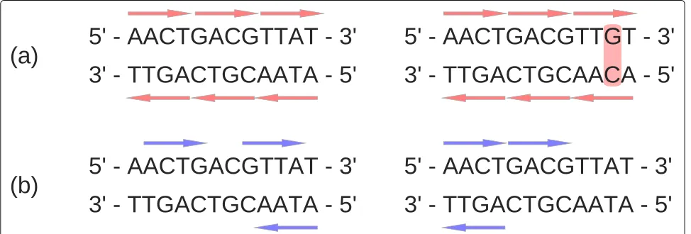
The bias caused by NGS samples can be illustrated by a simplified example in Fig. 1. Figure 1a shows two ficti-tious 12-bp genomes that differ by 1 bp (A-T ↔ G-C), and Fig. 1b shows two 12-bp genomes that are exactly the same. The dissimilarity measured by any reasonable alignment-free method between two genomes in Fig.1b should be 0 and is thus smaller than the dissimilarity between two genomes in Fig.1a. However, the dissimilar-ity between their NGS samples can show opposite results. For example, if the short reads (red arrows) in NGS sam-ples fully cover the two genomes in Fig.1a whereas the short reads (blue arrows) only partially cover the two genomes in Fig.1b, it is clear that the dissimilarity based on the two NGS samples in Fig. 1b is greater than the dissimilarity based on the two NGS samples in Fig. 1a. This apparent contradiction can be explained by differ-ent biases of NGS samples caused by differdiffer-ent sequencing depths.
Although Fig. 1 illustrates this bias by a simplified and extreme example, we used a real dataset of 21 pri-mates from [18] and simulated NGS samples to show this bias. In our previous study [14], we calculated pairwise ds2 and d2∗ using K = 5 to K = 14 where K is the length of thekmer with Markovian orderM = K −2 for the background sequences between these 21 primate
genomes and compared them with their pairwise evolu-tionary distances estimated by alignment-based methods. Our results showed that pairwiseds2andd∗2withK = 14 andM = 12 are highly correlated with their evolution-ary distances based on the alignments with Spearman correlation coefficients 0.979 for ds2 and 0.970 for d∗2 (Additional file1: Figures S1–S4).
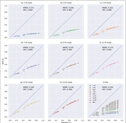
To study the influence of sequencing depths ond2s and d∗2, we simulated 8 NGS samples of different numbers of 150-bp Illumina reads (1 M, 3 M, 5 M, 7 M, 9 M, 11 M, 13 M, and 15 M) for each primate genome, correspond-ing to sequenccorrespond-ing depths from 0.05× to 0.75× (see the “Methods” section). A total 8 × 21 = 168 NGS sam-ples with different sequencing depths were generated and mixed together. We then calculated their pairwiseds2and d∗2values and compared them with the pairwised2sandd∗2 calculated based on their complete genomes. The result of ds2 using K = 14 and M = 12 is shown in Fig. 2. The results ofds2 using otherkmer lengths and Marko-vian orders are shown in Additional file1: Figure S5. The results of d∗2 using different kmer lengths are shown in Additional file1: Figures S6–S7. Bothds2andd2∗have been transformed to their corresponding similarity measures wheress2=1−2×d2sands∗2=1−2×d2∗.
As shown in Fig.2a–h, it is clear thatss2estimated from NGS samples is lower thanss2 estimated from genomes as all scatter points are below the dashed blue line across the diagonal and the bias, visualized as the gap between the scatter points and the diagonal, decreases when the sequencing depth increases. In addition, Fig.2a–h clearly illustrate thatss2calculated based on NGS strongly corre-lates withss2calculated based on the whole genomes if all samples have the same sequencing depth even when the sequencing depth is as low as 0.05× (1 M). The Spear-man correlation coefficients between ss2 based on NGS samples of 1 M reads and ss2 based on genomes is as
[image:3.595.57.544.540.705.2]Tanget al. Genome Biology (2019) 20:266 Page 4 of 17
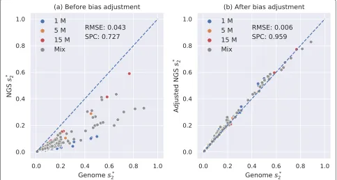
Fig. 2Relationship between pairwisess
2estimated by primate genomes and NGS samples usingK=14 andM=12 of different numbers of reads
without bias adjustment.X-axis is the pairwisess
2estimated by genomes, andY-axis is the pairwisess2estimated based on NGS samples.a–h
Relationship betweenss
2estimated by primate genomes andss2estimated based on NGS samples of only 1 M, 3 M, 5 M, 7 M, 9 M, 11 M, 13 M, or
15 M reads, respectively.iPairwisess
2estimated based on mixed NGS samples. NGS samples of different numbers of reads are colored accordingly.
“Mix” means two NGS samples have different numbers of reads (e.g., between 1 and 5 M or between 7 and 11 M) and is colored in gray. The root mean squared error (RMSE) and Spearman correlation coefficients (SPC) between pairwisess
2estimated based on NGS samples and genomes are
shown on each subplot
high as 0.969. However, if not all samples have the same sequencing depth, the Spearman correlation coefficient dropped significantly even when we analyzed more num-ber of reads in total, supported by comparing Figs.2a and i. In Fig. 2a, all samples have only 1 M reads whereas in Fig. 2i, each sample has a different number of reads
[image:4.595.56.541.86.561.2]that samples of 15 M reads have smaller bias than sam-ples of 1 M reads and therebyss2calculated from samples of 15 M reads will be generally greater than samples of 1 M reads regardless of their genomess2. This observa-tion supports our argument that bias caused by different sequencing depths markedly decrease the performance of alignment-free analysis based on NGS sequencing data. The same observation can be made ford2s using differ-entkmer lengths (Additional file1: Figure S5) and ford∗2 (Additional file1: Figures S6–S7). A more detailed results of the “Mix” label in Fig.2i was reported in Additional file
1: Figure S8a in which “Mix” was divided into more spe-cific labels such as “1 M and 5 M”, “1 M and 15 M,” and “5 M and 15 M.”
To show that this bias is a common problem for all alignment-free methods, we did the same analysis for another state-of-the-art alignment-free method Mash [5] which is based on Jaccard distance. We first calculated pairwise Mash distances based on 21 primate genomes usingK=14 (the samekmer length as we used fords2and d∗2),K=21 (defaultkmer length for Mash),K=31 (max-imum kmer length allowed by Mash), and sketch sizes s=103,s=105, ands=107and compared them with the pairwise evolutionary distances estimated by alignment-based methods. Additional file1: Figure S9 shows that the pairwise Mash distances and the evolutionary distances have the highest Spearman correlation coefficient of 0.984 when usingK=21 ands=107.
We then chose the kmer length K = 21 and sketch size s = 107 and compared Mash distances estimated
from primate genomes and Mash distances estimated from primate NGS samples. The results are shown in Additional file1: Figure S10, and Mash distance has been transformed to the corresponding Mash similarity that equals to 1 - Mash distance. Similar tos∗2 andss2, Mash similarity estimated from NGS samples is also lower than Mash similarity estimated from genomes, and this bias increases as the sequencing depth decreases as shown in Additional file 1: Figure S10a–h. As a consequence, the Spearman correlation coefficient (0.860) between Mash similarity based on genomes and Mash similarity based on NGS samples of 1 M to 15 M reads (Additional file1: Figure S10i) is even lower than the corresponding Spear-man correlation coefficient (0.943) based on NGS samples of only 1 M reads (Additional file1: Figure S10a).
As aforementioned, one solution is to downsample all NGS samples to have the same number of reads as the smallest sample, which is 1 M reads in this example, as shown in Fig.2a. This method does not adjust the bias of ss2 calculated based on NGS samples, but it controls that all samples have similar biases. The performance after downsampling is acceptable with Spearman corre-lation coefficient 0.969 (Fig. 2a) and is better than the performance without bias adjustment or downsampling
(Fig.2i). However, the vast majority of reads are discarded by downsampling, and thereby, much information is lost. For instance, in order to downsample a sample of 15 M reads to 1 M reads, we need to discard 93.3% of the reads in this sample.
Bias adjustment by a neural network regression model We characterize the bias adjustment process as a regres-sion problem that predicts the dissimilarity based on genomes from the dissimilarity based on NGS samples and their biases. It can be clearly seen in Fig. 2 and Additional file1: Figures S8a and S10 that the alignment-free dissimilarity between any pair of NGS samples d(ANGS,BNGS) is determined by the alignment-free
dis-similarity based on their genomesd(AG,BG)and the bias caused by each NGS sample Bias(ANGS)and Bias(BNGS):
d(ANGS,BNGS)=F(d(AG,BG), Bias(ANGS), Bias(BNGS))
In other words, if we know the function F, alignment-free dissimilarity between a pair of NGS samples, and their corresponding biases, then the alignment-free dis-similarity based on their genomes which is not biased by the sequencing depths in NGS samples can be pre-dicted. Although it is hard to infer a closed-form for-mula for function F for background-adjusted methods such as CVTree[1], d2s[2], and d∗2[2], a neural network regression model can be trained to approximate it, see the “Methods” section for more details about the defini-tion of Bias(ANGS), Bias(BNGS), and model training and
evaluation.
The correlation between the adjusted dissimilarity measures based on NGS samples and genomes of 21 primates is markedly increased
Tanget al. Genome Biology (2019) 20:266 Page 6 of 17
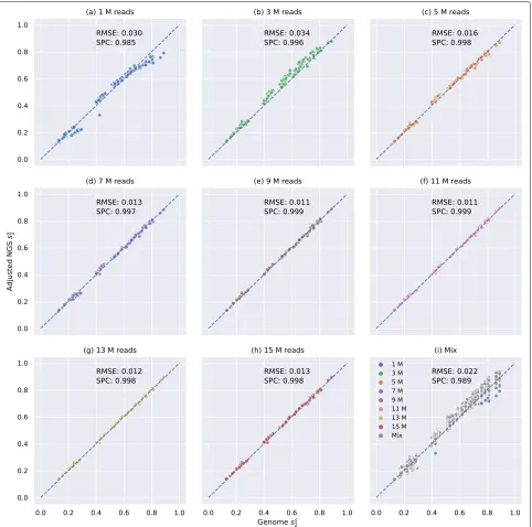
Fig. 3Relationship between pairwisess
2estimated by primate genomes and NGS samples usingK=14 andM=12 of different numbers of reads
with bias adjustment. X-axis is the pairwisess
2estimated by genomes and Y-axis is the pairwisess2estimated based on NGS samples after bias
adjustment.a–hshow the relationship betweenss
2estimated by primate genomes and adjustedss2based on NGS samples of only 1 M, 3M, 5 M, 7M,
9 M, 11 M, 13 M or 15 M reads, respectively.ishows pairwise adjustedss
2based on mixed NGS samples. NGS samples of different numbers of reads
are colored accordingly. ‘Mix’ means two NGS samples have different numbers of reads (e.g., between 1 M and 5 M or between 7 M and 11 M) and is colored in gray. The root mean squared error (RMSE) and Spearman correlation coefficients (SPC) between pairwisess
2estimated based on NGS
samples and genomes are shown on each subplot
NGSss2and genomess2, supported by the observation that most scatter points fall on the diagonal in Fig.3. In addi-tion, the root mean squared error was decreased, and the Spearman correlation coefficient was increased after bias adjustment. More importantly, Fig.3and Additional file1: Figures S8 and S11–13 revealed that our bias adjustment
[image:6.595.58.540.86.564.2]A possible explanation could be that the same number of reads cannot guarantee the same sequencing depth if genome lengths are different. Moreover, the bias might also be caused by other factors such as sequencing errors and sequencing bias that cannot be controlled by down-sampling. Therefore, we suggest always using our model to adjust the bias in the alignment-free analysis based on NGS sequencing data even when each sample has a similar number of reads to achieve better performance.
We also evaluated the performance of Skmer [8] on the same primate dataset using kmer length K = 21 and sketch size s = 107, which is a recent alignment-free method that corrects the formula of Mash dis-tance based on NGS samples by estimating the sequenc-ing depth and sequencsequenc-ing error rate. The relationship between the Skemr distances using the whole genomes and the Skmer distances using the NGS samples are shown in Additional file 1: Figure S14, and Skmer dis-tance has been transformed to the corresponding Skmer similarity that equals to 1 - Skmer distance. By compar-ing Additional file1: Figure S10a–h to the corresponding Additional file1: Figure S14a–h, we can see that Skmer adjusted Mash similarity by increasing its value estimated from NGS samples to compensate for the low sequenc-ing depths and sequencsequenc-ing errors as more points fall on diagonals in Additional file 1: Figure S14. However, Skmer decreased the Spearman correlation coefficients, especially when NGS samples have different sequenc-ing depths by comparsequenc-ing the coefficient of Mash (0.860) in Additional file 1: Figure S10i and the coefficient of Skmer (0.766) in Additional file1: Figure S14i. A possi-ble explanation could be that the formula that Skmer used in [8] to correct Mash distance by estimating sequenc-ing depth and sequencsequenc-ing error rate is not accurate when two NGS samples have different sequencing depths. As a comparison, Fig. 3 and Additional file 1: Figures S10 and S12 demonstrated that adjustedd2sandd∗2outperform Mash and Skmer in all circumstances, especially when the sequencing depth is low (<9 M reads) or samples have different sequencing depths.
The correlation between the adjusted dissimilarity measures based on NGS samples and genomes of 28 mammals is markedly increased
We tested our model fords2bias adjustment on an inde-pendent dataset of 28 mammals from [19]. In our pre-vious study [14], we have calculated pairwise ds2 using K = 14 and M = 12 between these 28 mammalian genomes and showed that their pairwise ds2 are highly correlated with their pairwise evolutionary distances esti-mated by alignment-based methods with Spearman cor-relation coefficient of 0.927, and the result is shown in Additional file1: Figure S15. We simulated 3 NGS sam-ples of different numbers of 150-bp Illumina reads (1 M,
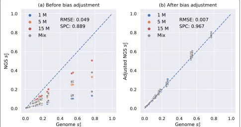
5 M, and 15 M) for each mammalian genome, corre-sponding to sequencing depths from 0.05× to 0.75×, resulting in a total of 28 × 3 = 84 samples (see the “Methods” section). We then calculated pairwise d2s between all 84 NGS samples, adjusted them using our neural network model and then compared them with the pairwiseds2calculated from their complete genomes. The result was transformed toss2and shown in Fig.4. It can be clearly seen in Fig.4a that pairwise NGSd2s was over-estimated before adjustment since all scatter points were below the diagonal whereas most scatter points after bias adjustment in Fig.4b fall on the diagonal, which proved that our model has successfully adjusted the bias ofd2s. In addition, the root mean squared error was decreased, and the Spearman correlation coefficient was increased after bias adjustment.
We next tested the performance of Mash and Skmer on the same mammalian dataset. We first calculated pair-wise Mash distances based on the 28 mammalian genomes using K = 14, K = 21, and K = 31 and sketch size s = 103, s = 105, and s = 107 and compared them with the pairwise evolutionary distances estimated by alignment-based methods. Additional file1: Figure S16 shows that pairwise Mash distances and the evolutionary distances have the highest Spearman correlation coeffi-cient of 0.943 when using K = 31 and s = 107. We then chosekmer lengthK = 31 and sketch sizes = 107 and compared Mash distance and Skmer distance esti-mated from mammalian genomes and estiesti-mated from NGS samples. The results are shown in Additional file1: Figure S17. The Spearman correlation coefficient (0.967) between adjustedds2based on NGS samples and genomes is significantly higher than that for Mash (0.789) and Skmer (0.688).
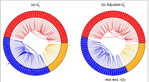
The accuracy on predicting continental origins of white oak NGS samples usingk-NN is markedly increased We tested our model ford∗2bias adjustment on a dataset of 92 white oak NGS samples collected from 3 conti-nents (North America, Asia, and Europe). In our previous study [12] , we downsampled each sample to 3 different sequencing quantities (50 Mbp, 100 Mbp, and 300 Mbp), corresponding to sequencing depths from 0.07×to 0.42×. At each sequencing quantity, samples were randomly divided into reference and query set, and for each sam-ple in the query set, we found its k-nearest neighbors (k-NN) measured by d∗2 with K = 12 and M = 10 in the reference set and predicted its continental origin by a majority vote approach (see the “Methods” section).k-NN accuracy at all these 3 sequencing quantities is shown in Additional file1: Table S1, and it can be clearly seen that the accuracy increases with sequencing quantity.
Tanget al. Genome Biology (2019) 20:266 Page 8 of 17
Fig. 4Relationship between pairwisess
2estimated usingK=14 andM=12 based on 28 mammalian genomes and NGS samples of different
numbers of reads.ashows the relationship before bias adjustment.bshows the relationship after bias adjustment for NGSss
2. The root mean
squared error (RMSE) was decreased and the Spearman correlation coeffient (SPC) between pairwise genomess
2and NGSss2was increased after bias
adjustment
300 Mbp dataset and mixed them together to build a new dataset of NGS samples with different sequencing quanti-ties. We predicted the continental origins of the samples in the query set using the same method, and results are shown at the top of Table1. Unsurprisingly, the accuracy was lower than even when we downsampled all samples to 50 Mbp (Additional file 1: Table S1) because a sam-ple from Asia might have smaller d∗2 to a sample from Europe of 300 Mbp than another sample from Asia of 50 Mbp, and it is likely to be misclassified. We used our model ford∗2 to adjust the bias and predicted their con-tinental origins again based on the dissimilarity after bias adjustment, and the prediction accuracy is shown at the bottom of Table 1. It is clear that our bias adjustment model was capable of increasing the accuracy markedly, especially when the reference size is small. It should be noticed that the accuracy after bias adjustment is higher than the accuracy by downsampling all samples to 50 Mbp or 100 Mbp, and it is comparable to the accuracy when all samples are of 300 Mbp, which shows that bias adjustment can achieve better performance than downsampling since the vast majority of reads are discarded by downsampling whereas bias adjustment still analyzes all the reads.
The prediction accuracy of Mash and Skmer was tested on the same oak dataset using K = 12, K = 21, and K = 31 and sketch sizes = 103,s = 105, ands = 107,
and results are shown in Additional file 1: Tables S2 and S3, respectively. It is clear that the adjusted d∗2 has higher prediction accuracy than Mash and Skmer, espe-cially when the reference size is small. For instance, when there are only 15 samples in the reference set, the adjusted d2∗ can still achieve an average prediction accuracy of 0.96 whereas the highest average prediction accuracies of Mash and Skmer usingK =31 ands= 107are 0.64 and 0.73, respectively.
The prediction accuracy of geographic origin at finer scales for white oak NGS samples is markedly increased
[image:8.595.56.541.88.344.2]Table 1Prediction accuracy usingk-NN on 92 white oak datasets of mixed sequence quantity based ond2∗before and after bias adjustment for different query sizes, reference sizes, and different numbers of neighborskused
Query size Reference size k= 1 k= 2 k= 3 k= 4 k=5 k= 6 k= 7 k= 8 k= 9 k= 10
Before bias adjustment
1 91 0.97 0.97 0.97 1.00 1.00 1.00 0.98 0.95 0.91 0.91
17 75 0.98 0.98 0.96 0.99 0.96 0.98 0.96 0.95 0.91 0.91
32 60 0.97 0.97 0.94 0.96 0.94 0.95 0.91 0.92 0.88 0.89
47 45 0.95 0.95 0.93 0.94 0.91 0.91 0.88 0.89 0.87 0.88
62 30 0.93 0.93 0.88 0.89 0.85 0.87 0.83 0.84 0.82 0.81
77 15 0.84 0.84 0.77 0.78 0.75 0.74 0.69 0.70 0.67 0.65
After bias adjustment
1 91 1.00 1.00 1.00 1.00 1.00 1.00 1.00 1.00 1.00 1.00
17 75 1.00 1.00 1.00 1.00 1.00 1.00 0.99 1.00 1.00 1.00
32 60 1.00 1.00 1.00 1.00 0.99 1.00 0.99 1.00 0.99 0.99
47 45 1.00 1.00 0.99 1.00 0.99 0.99 0.98 0.99 0.97 0.98
62 30 0.99 0.99 0.97 0.97 0.94 0.95 0.92 0.93 0.90 0.91
77 15 0.96 0.96 0.92 0.93 0.87 0.87 0.81 0.79 0.74 0.70
For each query sizes and reference sizes, the dataset was randomly split 100 times and an average prediction accuracy was calculated over 100 splits
most similar sample to 8 out of 16 European samples. The reason is that SRR2053099 (1414 Mbp) is one of the largest samples among all samples from Asia and SRR2053115 (1852 Mbp) is the largest sample among all samples from Europe, so they have the smallest biases in the samples
from Asia and Europe, respectively. Therefore, they are more likely to be predicted as the closest samples to other samples according tod2∗.
We adjusted the biases ofd∗2using Afann, and the results are shown in Fig.5b. It can be clearly seen that there is
[image:9.595.56.543.420.687.2]Tanget al. Genome Biology (2019) 20:266 Page 10 of 17
no sink node such as SRR2053099 and SRR2053115 in Fig.5a, which proves that the adjustedd∗2is not biased by sequencing depth. In order to show that bias adjustment can improve the prediction accuracy at finer geographic scales, we calculated the average distance between each sample and its closest sample according tod2∗before and after bias adjustment. In Fig.5, all samples are sorted by their longitude, so we define the distance between each sample and its closest sample based on their distance in the circular plots. For each sample, the minimum distance should be 1 if and only if its closest sample according to d∗2is next to it in the circular plots. The average distances between all 92 samples and their closest samples are 7.42 before bias adjustment and 5.85 after bias adjustment. A paired samplettest showed that the average distance after bias adjustment is significantly lower than before adjust-ment with apvalue of 0.023. Therefore, althoughd∗2based on NGS samples without downsampling or bias adjust-ment can successfully predict their continental origins, we proved that bias adjustment can further increase the prediction accuracy at finer geographic scales.
The correlation between the adjusted dissimilarity measures based on NGS samples and genomes of 67 vertebrates is markedly increased
Since our previous datasets all consist of sequencing reads coming from closely related species, we constructed a
dataset that contains samples from 67 vertebrates to eval-uate the performance of our method on diverse datasets. It contains vertebrate genomes of 67 species from 5 dif-ferent classes including fish, amphibians, reptiles, birds, and mammals. Among these 67 vertebrate genomes, we randomly selected 23, 22, and 22 genomes and simulated their NGS samples of 1 M, 5 M, and 15 M 150-bp Illu-mina reads, respectively, and mixed all 67 NGS samples together. The sequencing depths of all NGS samples range from 0.024×to 3.49×.
We then calculated pairwised∗2 andds2usingK = 14 andM= 12 between all 67 NGS samples with and with-out bias adjustment and compared them with the pairwise d2∗andds2calculated from their complete genomes. The result of d2∗ was transformed tos∗2 and shown in Fig 6. It can be demonstrated from Fig. 6 that our method markedly decreased the root mean squared error and increased the Spearman correlation coefficient from 0.727 to 0.959. The result ofds2was transformed toss2and shown in Additional file1: Figure S18, and the bias adjustment ofds2increased the Spearman correlation coefficient from 0.701 to 0.935.
The performance of Mash and Skmer using K = 31 ands = 107 was tested on the same vertebrate dataset and shown in Additional file 1: Figure S19. The Spear-man correlation coefficients between adjustedd2∗(0.959) and adjustedds2(0.935) based on vertebrate NGS samples
[image:10.595.56.540.435.694.2]and genomes are significantly higher than that for Mash (0.747) and Skmer (0.735).
Running time and memory
Although background-adjusted alignment-free methods such asCVTree[1],d2s [2], andd∗2 [2] have been shown to achieve better performance than simple Manhattan andEuclideandistances [10,12,14,16,17], their applica-tions have been limited due to the high time and memory cost in the random background removing step. To over-come this bottleneck, we improved the speed and memory usage of background-adjusted methods in Afann by hash-ing, multi-threadhash-ing, and vectorization and compared it with our previous program Cafe [14].
Both tools were used to calculate the pairwised2s, d2∗, and CVTree among the white oak datasets of 92 NGS samples with 300 Mbp sequencing quantity using K = 12 and M = 10 and among the primate dataset of 21 genomes usingK = 14 and M = 12. Comparisons of time and memory based on white oak datasets and pri-mate dataset were shown in Table 2and Additional file
[image:11.595.56.289.480.671.2]1: Table S4, respectively. The total time was divided into kmer counting time and dissimilarity calculation time. It can be clearly seen in Table2that the total speedup ratio of Afann is around 100× for all 3 background-adjusted methods whereas the memory usage is only one fifth of
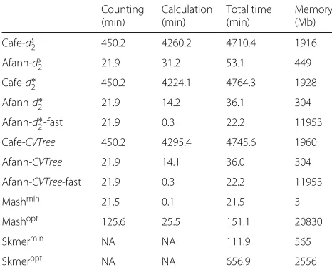
Table 2kmer counting time, dissimilarity calculation time, and total time as well as memory usage used by Cafe and Afann to calculate the pairwiseds2,d∗2, andCVTreeusingK=12 and M=10 among a dataset of 92 white oak NGS samples of 300 Mbp
Counting (min)
Calculation (min)
Total time (min)
Memory (Mb)
Cafe-ds
2 450.2 4260.2 4710.4 1916
Afann-ds
2 21.9 31.2 53.1 449
Cafe-d∗2 450.2 4224.1 4764.3 1928
Afann-d∗2 21.9 14.2 36.1 304
Afann-d∗2-fast 21.9 0.3 22.2 11953 Cafe-CVTree 450.2 4295.4 4745.6 1960
Afann-CVTree 21.9 14.1 36.0 304
Afann-CVTree-fast 21.9 0.3 22.2 11953
Mashmin 21.5 0.1 21.5 3
Mashopt 125.6 25.5 151.1 20830
Skmermin NA NA 111.9 565
Skmeropt NA NA 656.9 2556
Afann-d∗2-fast and Afann-CVTree-fast stand for the fast mode ofd∗2andCVTree supported in Afann. Running time and memory usage of Mash and Skmer were also included. Mashminand SkmerminusedK=12 ands=103which require the minimum computing power. Mashoptand SkmeroptusedK=31 ands=107 which have the optimal performance among Mash and Skmer using different combinations ofkmer lengths and sketch sizes as shown in Additional file1: Table S2 and Table S3
the memory of Cafe. Afann also supports fast calculation mode ford∗2andCVTreewhich further increases the cal-culation speed by using more memory. The memory usage isO(4K) for normal mode andO(N ×4K) for the fast mode whereK is thekmer length andN is the number of samples. It should be noticed that the counting time is O(N×4K)whereas the calculation time isO(N2×4K); the total speedup ratio will thereby be close to the speedup ratio of dissimilarity calculation as the number of samples N increases. We suggest using fast mode when memory allows. For example, it is common to compare the pairwise dissimilarity among thousands of bacterial genomes using small kmer length 5 or 6 which does not require much memory, then the speedup ratio of fast mode can be more than 5000×.
The running time and memory usage of other fast alignment-free tools Mash [5] and Skmer [8] on the same oak NGS and primate genome datasets were also calcu-lated and reported in Table2and Additional file1: Table S4, respectively. The running time and memory usage of an alignment-free genome comparison tool FFP [3] on the primate genome dataset usingK = 16 as suggested in [3] were reported in Additional file1: Table S4. It should be noticed that the running time of Mash and Skmer using K = 12 nad s = 103 for oak NGS dataset and K = 14 and s = 103 for primate genome dataset was only included to test their speed when using the same kmer length asd∗2andds2. In practice,kmer length shorter than 21 is not recommended for Mash and Skmer [8]. We can see in Table 2 and Additional file 1: Table S4 that Cafe calculatesds2,d2∗, andCVTreemuch slower than Mash, Skmer, and FFP whereas Afann is capable of cal-culatingd2s,d∗2, andCVTreein a comparable amount of time as Mash, Skmer, and FFP. The pairwise dissimilarity measures among primate genomes calculated by different methods were compared with their evolutionary distances estimated by alignment-based methods in [18] and shown in Additional file1: Figure S20. All dissimilarity measures except FFP are highly correlated with the evolutionary dis-tance with Spearman correlation coefficients higher than 0.95 which demonstrated the applicability of alignment-free methods in genome comparisons. However, our eval-uations based on different independent datasets in previ-ous sections showed that Afann significantly outperforms others in comparing NGS samples.
Discussion
Tanget al. Genome Biology (2019) 20:266 Page 12 of 17
the stochastic distribution of short reads [4, 8, 12]. In this study, we showed that this bias could signifi-cantly decrease the performance of alignment-free analy-sis based on NGS samples of different sequencing depths by investigating four independent datasets. For the pri-mate, mammalian, and vertebrate datasets, the correlation between pairwise NGS dissimilarity and pairwise genome dissimilarity dropped markedly if NGS samples of differ-ent numbers of reads were mixed together. For the white oak dataset, thek-NN prediction accuracy of their conti-nental origins based on a dataset of samples with 50 M, 100 M, and 300 M sequencing quantity is even much lower than the accuracy based on a dataset of all samples with only 50 M sequencing quantity.
This problem was previously solved by downsampling [12] or modifying the specific dissimilarity formula by estimating the sequencing depth and sequencing error rate [4, 8]. However, the first method discards the vast majority of reads that could have been informative, and the second method depends on the estimation of sequenc-ing depth and sequencsequenc-ing error rate and cannot be gener-alized to adjust the bias for other alignment-free methods calculated by a different formula. In addition, it can be extremely hard to adjust the formula of several compli-cated background-adjusted methods such as CVTree[1], ds2[2], andd∗2[2].
Therefore, we introduced a de novo method in this study to adjust bias without estimating the sequenc-ing depth or sequencsequenc-ing error rate explicitly by definsequenc-ing Bias(ANGS) = d(ANGS,ARNGS). This bias estimator will
increase as the sequencing depth decreases or sequencing error rate increases and thus implicitly capture informa-tion from sequencing depth and sequencing error rate. Therefore, bias adjustment could be characterized as a regression problem that usesd(ANGS,BNGS), Bias(ANGS),
and Bias(BNGS) to predict d(AG,BG). Two neural net-work regression models were trained fords2andd2∗ sepa-rately using the primate dataset. Our results showed that bias was successfully adjusted for NGS samples of differ-ent sequencing depth and calculated by using differdiffer-ent kmer length, supported by the large improvement of root mean squared error and Spearman correlation coefficient between dissimilarity based on NGS samples after bias adjustment and dissimilarity based on genomes.
Without changing any parameters, the performance of our models was tested on 3 independent datasets. A 28 mammalian dataset was used to test our bias adjustment model fords2. Each genome was simulated to 3 NGS sam-ples of 1 M, 5 M, and 15 M Illumina 150-bp reads and mixed together. Pairwise d2s values using K = 14 and M = 12 between all 84 samples were calculated with-out and with bias adjustment and compared with pairwise genomed2s. The results showed that our method success-fully adjusted the bias and greatly improved both root
mean squared error and Spearman correlation coefficient. A 92 white oak dataset was used to test our bias adjust-ment model for d∗2. We randomly selected 30 samples from the 50 Mbp dataset, 31 samples from the 100 Mbp dataset, and 31 samples from the 300 Mbp dataset and mixed them together. Pairwised∗2values usingK=12 and M = 10 between all 92 samples were calculated without and with bias adjustment, andk-NN was used to predict the continental origins of test samples based ond∗2. Our result showed that the prediction accuracy of the mixed dataset usingk-NN is even lower than that using a dataset of all 50 Mbp samples before bias adjustment. After bias adjustment, the k-NN accuracy markedly increased and was comparable to the accuracy based on a dataset of all 300 Mbp samples. In addition, we proved that bias adjust-ment could increase the accuracy of prediction not only at continental level but also at finer geographic scales. At last, a 67 vertebrate dataset consisting of species from 5 different classes was used to demonstrate the reliability of our method on datasets composed of diverse species. In all datasets, our method outperformed other alignment-free methods including Mash [5] and Skmer [8] in terms of the Spearman correlation coefficient and prediction accuracy. It should be noticed that while our bias adjust-ment method is capable of successfully predicting the alignment-free dissimilarity based on genomes regardless of the chosenkmer length, it is, nevertheless, important to choose a properkmer length so that the alignment-free dissimilarity based on genomes is highly correlated with their evolutionary distance. For instance, while Additional file 1: Figure S11 shows that our model successfully adjusted the bias of ds2 using K = 5 to K = 13 based on primate NGS samples, it can be clearly seen in Additional file1: Figure S4 that the correlation between d2sbased on primate genomes and their evolutionary dis-tance is lower than 0.90 whenK <10 is used. Therefore, even if our model can adjust the bias of K < 10, the performance might not increase as we expected. There have been several investigations into the choice of optimal kmer length [2,3,20,21]. In practice, shorterkmers are optimal when sequences are short or obviously different, whereas longerkmers should be used when sequences are from very closely related species in order to reduce the probability that akmer commonly appear in a sequence by chance [2,3,5,20].
using more samples from different species with more variant sequencing depths to further improve the per-formance. In addition, since our bias adjustment method only relies on the alignment-free dissimilarity calculated between ANGS and ARNGS without estimating
sequenc-ing depths and sequencsequenc-ing error rates or considersequenc-ing the actual formula of the dissimilarity measures, it can be easily generalized to adjust the bias of all alignment-free dissimilarity measures by training their own regression models. In this paper, we showed the success of our bias adjustment model for two background-adjusted methods ds2 and d2∗; the framework developed in this paper can be easily adapted to adjust bias in other alignment-free dissimilarity measures.
Conclusion
Afann is a fast tool to calculate background-adjusted alignment-free dissimilarity measuresCVTree,d∗2, andd2s between genome sequences and NGS samples. In addi-tion, it can adjust the biases caused by NGS samples of different sequencing depths ford∗2andds2without down-sampling or estimating the sequencing depth. Our results showed that the adjusted d2∗ and ds2 are not biased by sequencing depth and can significantly increase the per-formance of studies based on NGS samples.
Methods
See Appendix A of Additional file1for more details about different alignment-free dissimilarity measures including CVTree[1],d2s[2], andd∗2[2].
Genomic datasets and simulation of NGS samples
The primate dataset consists of 21 complete primate genome sequences downloaded from NCBI. In [18], the author estimated the evolutionary distances among 186 primates based on the alignment of 54 nuclear gene regions. In our previous study [14], we found 21 com-plete representative genomes on NCBI among these 186 primates and demonstrated that their pairwiseds2andd∗2 with K = 14 and M = 12 are highly correlated with their evolutionary distances estimated in [18]. The species names, assembly accession numbers, and total sequence lengths of these 21 primate genomes are shown in Addi-tional file 1: Table S5. For each genome, we used ART [22] to simulate different numbers of Illumina HiSeq 2500 reads of length 150 bp with default sequencing error pro-file. We produced 8 different datasets with 1 M, 3 M, 5 M, 7 M, 9 M, 11 M, 13 M, and 15 M reads for each NGS sam-ple. We then mixed all 21×8 = 168 NGS samples to generate a new dataset of primate NGS samples.
Similarly, the mammalian dataset consists of 28 com-plete vertebrate genome sequences downloaded from NCBI, with evolutionary distances calculated by the alignment-based method in [19]. The species names,
assembly accession numbers, and total sequence lengths of these 28 mammalian genomes are shown in Additional file1: Table S6. For each genome, we used ART [22] to simulate different numbers of Illumina HiSeq 2500 reads of length 150 bp with default sequencing error profile. We produced 3 different datasets with 1 M, 5 M, and 15 M reads for each NGS sample. We then mixed all 28×3=84 NGS samples to generate a new dataset of mammalian NGS samples.
The white oak tree dataset consists of whole-genome shotgun (WGS) sequencing data of 92 white oaks from North America, Europe, and Asia with sequencing quan-tity ranging from 379 to 1852 Mbp from NCBI BioProject PRJNA269970 [23]. The run accession numbers, number of bases, and continental origins for these 92 samples are shown in Additional file1: Table S7. We downsampled all 92 samples to produce 3 different datasets with 50 Mbp, 100 Mbp, and 300 Mbp, for each sample, respectively. Then, we randomly chose 30 samples from the 50 Mbp dataset, 31 samples from the 100 Mbp dataset, and 31 samples from the 300 Mbp and mixed them together to generate a new dataset of 92 NGS samples with differ-ent sequencing quantities. All samples were divided into 3 geographic categories (North America, Europe, and Asia) based on their continental origins.
The vertebrate dataset consists of 67 complete verte-brate genome sequences downloaded from NCBI. The species are from 5 different classes, including 15 fish, 7 amphibians, 15 reptiles, 15 birds, and 15 mammals. All 15 species were randomly selected from the correspond-ing classes except for amphibian where there are only 7 amphibian complete genome sequences available on NCBI, and thereby, they were all included in the dataset. The species names, classes, assembly accession numbers, and total sequence lengths of these 67 vertebrate genomes are shown in Additional file1: Table S8. Among these 67 vertebrate genomes, we randomly selected 23, 22, and 22 genomes and simulated their NGS samples of 1 M, 5 M, and 15 M 150 bp Illumina reads, respectively, by ART [22] and mixed them together to generate a dataset of 67 vertebrate NGS samples.
Developing a bias adjustment model
For any pair of NGS samples, their alignment-free dis-similairtyd(ANGS,BNGS)is determined by three variables,
which are the alignment-free dissimilairty based on their genomesd(AG,BG)and the bias caused by each sample Bias(ANGS)and Bias(BNGS):
d(ANGS,BNGS)=F(d(AG,BG), Bias(ANGS), Bias(BNGS))
(1)
Tanget al. Genome Biology (2019) 20:266 Page 14 of 17
Bias(ANGS)=d
ANGS,ARNGS
(2)
where ANGS is the original NGS sample and ARNGS is a
mapped NGS sample that each read in it is a reverse com-plementary mapping of a read in the original NGS sample. For example, the NGS sample in the left of Fig. 1a has reads {AACT, GACG, TTAT, ATAA, CGTC, AGTT}, and its correspondingARNGScan be inferred by mapping each read inANGSto its reverse complementary read and thus
is {AGTT, CGTC, ATAA, TTAT, GACG, AACT}, which is exactly the same asANGS. The NGS sample in the left
of Fig.1b has reads {ACTG, GTTA, ATAA}, and itsARNGS should be {CAGT, TAAC, TTAT} accordingly, which is apparently different fromANGS.
Given an dissimilarity measure, such as ds2 or d∗2, the Bias(ANGS) can then be calculated between ANGS and
ARNGS. We expect that Bias(ANGS) will increase as the
sequencing depth of ANGS decreases or the sequencing
error rate increases, as shown in Fig. 1b. The advantage of defining Bias(ANGS)in this way is that we do not need
to estimate sequencing depth or sequencing error rate explicitly, but this information has already been implicitly considered when we compareANGSwithARNGS.
Given d(AG,BG), d(ANGS,BNGS) will increase as
Bias(ANGS) or Bias(BNGS)increases, as shown in Fig. 2i
that samples of high sequencing depth and thus low bias (red points) have higher NGSss2(lower NGSds2) than sam-ples of low sequencing depth and thus high bias (blue points) even when their genomesof interest are the same. In addition, if Bias(ANGS)and Bias(BNGS)do not change,
d(ANGS,BNGS) will increase as d(AG,BG) increases, as shown in Fig.2a–h. Since NGS samples in the same sub-plot have the same number of reads and thus have similar Bias(ANGS)and Bias(BNGS), their pairwised(ANGS,BNGS)
value increases withd(AG,BG).
Because of this partial monotonic relationship between d(ANGS,BNGS) and d(AG,BG) given Bias(ANGS) and
Bias(BNGS), Eq. (1) can be rewritten as:
d(AG,BG)=G(d(ANGS,BNGS),Bias(ANGS), Bias(BNGS))
(3)
whereGis a general function. Therefore, the bias adjust-ment process can be characterized as a regression prob-lem that is capable of predicting the real genome dissim-ilarity d(AG,BG) between any pair of NGS samples. To solve this supervised learning problem, we can first train our regression models on datasets of known d(AG,BG), d(ANGS,BNGS), Bias(ANGS), and Bias(BNGS). Then, for
any new pair of NGS samples, we first calculate their d(ANGS,BNGS), Bias(ANGS), and Bias(BNGS)and use our
model to predict its d(AG,BG). After bias adjustment, our sequence comparison can be based on the predicted unbiasedd(AG,BG)instead of biasedd(ANGS,BNGS).
Model training and evaluation
Creating training samples
We trained 2 neural network regression models that are widely used to solve nonlinear regression problems fords2 andd∗2separately using the 21 primate dataset. Instead of training on NGS samples we generated previously to plot Fig.2, we generated a new dataset by simulating 8 NGS samples of different number of reads (1 M, 3 M, 5 M, 7 M, 9 M, 11 M, 13 M, and 15 M) for each genome again and mixed them together. The samples are denoted fromP1NGS to PNGS168 , respectively. We describe how we trained the bias adjustment model ford2sin the following section. The same training method was used ford∗2and can be easily generalized for other alignment-free methods.
For each pair of NGS samples PiNGS and PjNGS, we calculated their NGS dissimilarity ds2PiNGS,PNGSj , their genome dissimilarity ds2PiG,PjG, BiasPiNGS, and Bias
PjNGS
using kmer length from 5 to 14 and Markovian order = k− 2. For each kmer length, there are 168 × 167 = 28, 056 pairs, so that Xk will be a matrix of dimension 28, 056× 3 and yk will be a vec-tor of length 28,056 as shown below. To ensure that our model can train BiasPiNGS and BiasPNGSj symmet-rically, bothd2sPNGSi ,PjNGS andds2PjNGS,PiNGSwere included in the training samples, which was verified after model training and shown in Additional file1: Figure S21. In order to build a regression model that is capable of adjusting the bias for differentkmer lengths, we concate-nated Xk fromX5 to X14 vertically and concatenated yk fromy5toy14. Therefore, our finalX=
X5T,X6T. . .X14TT is a 280, 560× 3 matrix and y = yT
5,yT6,. . .yT14
T is a 280, 560×1 vector.
⎡ ⎢ ⎢ ⎢ ⎢ ⎢ ⎢ ⎢ ⎢ ⎢ ⎢ ⎢ ⎢ ⎢ ⎢ ⎢ ⎢ ⎢ ⎢ ⎢ ⎢ ⎣ ds 2 P1 NGS,PNGS2
BiasP1 NGS
BiasP2 NGS
d2sP1NGS,PNGS3 BiasPNGS1 BiasP3NGS d2sP1NGS,PNGS4 BiasPNGS1 BiasP4NGS
..
. ... ...
d2sP1NGS,PNGS168 BiasP1NGS BiasP168NGS d2sP2NGS,PNGS1 BiasPNGS2 BiasP1NGS d2sP2NGS,PNGS3 BiasPNGS2 BiasP3NGS d2sP2NGS,PNGS4 BiasPNGS2 BiasP4NGS
..
. ... ...
d2sP168NGS,PNGS167 BiasPNGS168 BiasP167NGS
⎤ ⎥ ⎥ ⎥ ⎥ ⎥ ⎥ ⎥ ⎥ ⎥ ⎥ ⎥ ⎥ ⎥ ⎥ ⎥ ⎥ ⎥ ⎥ ⎥ ⎥ ⎦ Xk ∼ ⎡ ⎢ ⎢ ⎢ ⎢ ⎢ ⎢ ⎢ ⎢ ⎢ ⎢ ⎢ ⎢ ⎢ ⎢ ⎢ ⎢ ⎢ ⎢ ⎢ ⎢ ⎣ ds 2 P1 G,P2G
d2sP1G,P3G d2sP1G,P4G
.. . ds2P1G,P168G
d2sP2G,P1G d2sP2G,P3G d2sP2G,P4G
.. . ds2P168G ,P167G
⎤ ⎥ ⎥ ⎥ ⎥ ⎥ ⎥ ⎥ ⎥ ⎥ ⎥ ⎥ ⎥ ⎥ ⎥ ⎥ ⎥ ⎥ ⎥ ⎥ ⎥ ⎦ yk
Training samples augmentation
is no bias in NGS samples, then the alignment-free dis-similarity based on NGS samples should be equal to the dissimilarity based on their genomes (d(ANGS,BNGS) =
d(AG,BG) ⇐⇒ Bias(ANGS) = Bias(BNGS) = 0).
Therefore, we defined a hyperparameter augmentation ratio asr, and randomly simulatedd1todm(di∼U(0, 1)) and concatenatedXAandyAshown as below to our train-ing samplesX andy, respectively, to fit our model. The sizes ofXAandyAwere determined by the size of training samples and augmentation ratiorwherem= |X| ×r.
⎡ ⎢ ⎢ ⎢ ⎢ ⎢ ⎣
d1 0 0
d2 0 0
d3 0 0
.. . ... ... dm 0 0
⎤ ⎥ ⎥ ⎥ ⎥ ⎥ ⎦
XA ∼
⎡ ⎢ ⎢ ⎢ ⎢ ⎢ ⎣
d1
d2
d3
.. . dm
⎤ ⎥ ⎥ ⎥ ⎥ ⎥ ⎦
yA
Hyperparameter tuning and evaluation
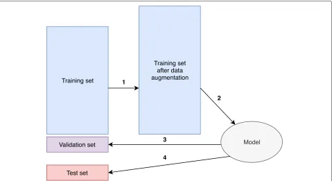
A neural network regression model with ReLU activation (sklearn.neural_network.MLPRegressor), was trained and a grid search algorithm was implemented to find the opti-mal combination of hyperparameters such as hidden layer sizes, regularization term, and augmentation ratio. The workflow is described below and also shown in Fig.7.
1. Twenty-eight thousand fifty-six (10%) samples were randomly selected as a held-out test set. The remaining 252,504 (90%) samples were used as a training set.
2. A given combination of hyperparameters was chosen. Steps 3–4 were repeated 10 times, and the averageR2
under this combination of hyperparameters were calculated (10-fold cross-validation).
3. Ten percent of the samples from the training set were randomly chosen as a validation set, the other 90% of the samples were first augmented as aforementioned and then used to fit our model. 4. The trained model was used to predictd(AG,BG)for
the validation set, andR2was calculated.
5. Repeat steps 2–4 with different hyperparameters, and the optimal combination of hyperparameters with the highest averageR2was chosen
(hyperparameter tuning).
6. The optimal combination of hyperparameters was chosen, and trained on all training set, and the final model was used to predictd(AG,BG)for the held-out
test set andR2was calculated (evaluation).
Finally, the combination of hyperparameters with the highest cross-validation score was chosen (1 hidden layer with 2000 neurons, regularization term 0.0001, and aug-mentation ratio 2) and tested on the held-out test data
Fig. 7Diagram of hyperparameter tuning and evaluation. (1) Trainig set is augmented. (2) Training set after data augmentation is used to fit the model. (3) The trained model is used to predictd(AG,BG)for the validation set. For each combination of hyperparameters, we repeated steps 1–3
ten times to calculate the averageR2, and the combination of hyperparameters with the highest averageR2was chosen. (4) After hyperparameter
[image:15.595.61.540.423.684.2]Tanget al. Genome Biology (2019) 20:266 Page 16 of 17
with an R2 value 0.98 fords
2 and 0.99 for d∗2. The final
models for ds2andd2∗ were then used to adjust the bias for primate, mammalian, vertebrate, and white oak NGS datasets. It should be mentioned that altoughd(AG,BG) andd(BG,AG)were almost identical as shown in Addi-tional file1: Figure S21, we take the average ofd(AG,BG) andd(BG,AG)as the final predicted dissimilarity between A and B to strictly satisfy the symmetry property.
White oak continental origin prediction byk-NN andd∗2
For each sequencing quantity (50, 100, and 300 Mbp), we first calculated the pairwised∗2usingK=12 andM=10 between each pair of samples in the dataset. Then, 92 samples were randomly divided into the reference set and query set. The number of samples in the reference set ranges from 91 (leave-one-out), 77, 60, 45, and 30 to 15. For each sample in the query set, we found itsk-nearest (k=1–10) neighbors measured byd2∗in the reference set and predicted its continental origin by a majority vote. For each reference size, we split 100 times and the pre-diction accuracy was averaged over 100 splits and shown in Additional file1: Table S1. We then randomly selected 30 samples from the 50 Mbp dataset, 31 samples from the 100 Mbp dataset, and the 300 Mbp dataset as a mixed dataset. The same prediction method was used, and accu-racies with and without bias adjustment were shown in Table1.
Supplementary information
Supplementary informationaccompanies this paper at https://doi.org/10.1186/s13059-019-1872-3.
Additional file 1: Supplementary methods, supplementary figures, supplementary tables.
Additional file 2: Review history.
Peer review information
Andrew Cosgrove was the primary editor of this article and managed its editorial process and peer review in collaboration with the rest of the editorial team.
Acknowledgements
This research utilized resources of high-performance computing (HPC), which is supported by the University of Southern California.
Review history
The review history is available as Additional file2
Authors’ contributions
KT, JR, and FS conceived the project. KT developed the algorithm,
implemented the software, carried out the computational analyses, and wrote the paper. JR revised the paper. FS led the project and finalized the paper. All authors agree to the content of the final paper. All authors read and approved the final manuscript.
Funding
This research was partially supported by the US National Science Foundation (NSF) [DMS-1518001] and National Institutes of Health (NIH) [R01GM120624, 1R01GM131407].
Availability of data and materials
Afann software is publicly available athttps://github.com/GeniusTang/Afann [24] under the terms of USC-RL v1.0. Afann is written in C++ and Python and has been tested on Unix and Mac OS X. The version of software used in the manuscript is deposited in Zenodohttps://doi.org/10.5281/zenodo.3483847 [25]. The detailed description of genomic datasets and simulation methods used in our experiments is provided in “Genomic datasets and simulation of NGS samples” section.
Ethics approval and consent to participate Not applicable.
Consent for publication Not applicable.
Competing interests
The authors declare that they have no competing interests.
Received: 2 May 2019 Accepted: 29 October 2019
References
1. Qi J, Luo H, Hao B. CVTree: a phylogenetic tree reconstruction tool based on whole genomes. Nucleic Acids Res. 2004;32(suppl_2):W45–7. 2. Reinert G, Chew D, Sun F, Waterman MS. Alignment-free sequence
comparison (i): statistics and power. J Comput Biol. 2009;16(12):1615–34. 3. Sims GE, Jun S-R, Wu GA, Kim, S-H. Alignment-free genome comparison with feature frequency profiles (FFP) and optimal resolutions. Proc Natl Acad Sci. 2009;106(8):2677–82.
4. Fan H, Ives AR, Surget-Groba Y, Cannon CH. An assembly and alignment-free method of phylogeny reconstruction from next-generation sequencing data. BMC Genomics. 2015;16(1):522. 5. Ondov BD, Treangen TJ, Melsted P, Mallonee AB, Bergman NH, Koren S,
Phillippy AM. Mash: fast genome and metagenome distance estimation using Minhash. Genome Biol. 2016;17(1):132.
6. Zielezinski A, Vinga S, Almeida J, Karlowski WM. Alignment-free sequence comparison: benefits, applications, and tools. Genome Biol. 2017;18(1):186.
7. Ren J, Bai X, Lu YY, Tang K, Wang Y, Reinert G, Sun F. Alignment-free sequence analysis and applications. Ann Rev Biomed Data Sci. 2018;1: 93–114.
8. Sarmashghi S, Bohmann K, Gilbert MTP, Bafna V, Mirarab S. Skmer: assembly-free and alignment-free sample identification using genome skims. Genome Biol. 2019;20(1):34.
9. Zielezinski A, Girgis HZ, Bernard G, Leimeister C-A, Tang K, Dencker T, Lau AK, Röhling S, Choi J, Waterman MS, et al. Benchmarking of alignment-free sequence comparison methods. Genome Biol. 2019;20(1): 144.
10. Jiang B, Song K, Ren J, Deng M, Sun F, Zhang X. Comparison of metagenomic samples using sequence signatures. BMC Genomics. 2012;13(1):730.
11. Song K, Ren J, Zhai Z, Liu X, Deng M, Sun F. Alignment-free sequence comparison based on next-generation sequencing reads. J Comput Biol. 2013;20(2):64–79.
12. Tang K, Ren J, Cronn R, Erickson DL, Milligan BG, Parker-Forney M, Spouge JL, Sun F. Alignment-free genome comparison enables accurate geographic sourcing of white oak DNA. BMC Genomics. 2018;19(1):896. 13. Karlin S, Burge C. Dinucleotide relative abundance extremes: a genomic
signature. Trends Genet. 1995;11(7):283–90.
14. Lu YY, Tang K, Ren J, Fuhrman JA, Waterman MS, Sun F. CAFE: aCcelerated Alignment-FrEe sequence analysis. Nucleic Acids Res. 2017;45(W1):W554–9.
15. Ahlgren NA, Ren J, Lu YY, Fuhrman JA, Sun F. Alignment-free oligonucleotide frequency dissimilarity measure improves prediction of hosts from metagenomically-derived viral sequences. Nucleic Acids Res. 2016;45(1):39–53.
16. Tang K, Lu YY, Sun F. Background adjusted alignment-free dissimilarity measures improve the detection of horizontal gene transfer. Front Microbiol. 2018;9:711.
18. Perelman P, Johnson WE, Roos C, Seuánez HN, Horvath JE, Moreira MAM, Kessing B, Pontius J, Roelke M, Rumpler Y, et al. A molecular phylogeny of living primates. PLOS Genet. 2011;7(3):e1001342. 19. Miller W, Rosenbloom K, Hardison RC, Hou M, Taylor J, Raney B,
Burhans R, King DC, Baertsch R, Blankenberg D, et al. 28-way vertebrate alignment and conservation track in the UCSC genome browser. Genome Res. 2007;17(12):1797–808.
20. Wu T-J, Huang Y-H, Li L-A. Optimal word sizes for dissimilarity measures and estimation of the degree of dissimilarity between DNA sequences. Bioinformatics. 2005;21(22):4125–32.
21. Bai X, Tang K, Ren J, Waterman M, Sun F. Optimal choice of word length when comparing two Markov sequences using aχ2-statistic. BMC
Genomics. 2017;18(6):732.
22. Huang W, Li L, Myers JR, Marth GT. Art: a next-generation sequencing read simulator. Bioinformatics. 2011;28(4):593–4.
23. ID 269970 - BioProject - NCBI. USDA Forest Service.https://www.ncbi.nlm. nih.gov/bioproject/PRJNA269970. Accessed 13 Oct 2019.
24. Tang K, Ren J, Sun F. Afann: bias adjustment for alignment-free sequence comparison based on sequencing data using neural network regression. Github. 2019.https://github.com/GeniusTang/Afann. Accessed 13 Oct 2019.
25. Tang K, Ren J, Sun F. Afann: bias adjustment for alignment-free sequence comparison based on sequencing data using neural network regression. Zenodo. 2019.https://doi.org/10.5281/zenodo.3483847. Accessed 13 Oct 2019.
Publisher’s Note