Analysis of Data Prediction Algorithms in Wireless Sensor Networks

Technology (IJRASET)

©IJRASET: All Rights are Reserved

176

Analysis of Data Prediction Algorithms in

Wireless Sensor Networks

R.Rebecca1, S. Kalaivani2 1,2

Department Of Electronicsand Communication Engineering B. S. Abdur Rahman University Chennai, India

Abstract-- Wireless Sensor Network (WSNs) is a network that consists of several sensor nodes which are resource constrained. The nodes gather data from external environment and send data to base station. The major problem in the sensor node is the energy consumption during transmission. To address this issue data prediction is used in this paper. Derivative Based Prediction Algorithm(DBP), Auto Regressive Prediction Algorithm(AR), Moving Average Prediction Algorithm(MA) and Auto Regressive Integrated Moving Average Prediction Algorithm(ARIMA) also is analyzed and observed that ARIMA model provides least RMSE and much suitable for data prediction in sensor network .

Index Terms— Wireless sensor networks, data prediction, energysaving, network life time.

I. INTRODUCTION

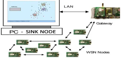
Wireless sensor network are spatially distributed sensors that have freedom to govern itself or control its own affairs[1]. These sensors senses the environmental condition and send the sensed data to sink node through the network. Sink node collect all the sets of data for further processing . These sensor node consumes more power for communicating, data processing and sensing. Among which communication causes high power consumption. Since the wireless sensor node is kept in a location which is hard to reach , so it is inconvient to change the battery regularly.This high power consumption problem can be reduced by reducing the amount of data sent to the destination node. Different data reduction techniques have been developed to overcome these problems. Data compression, data prediction and inter networking process are the different types of techniques developed to reduce the data sent to the sink node.To reduce the amount of data received in the source node data compression technique is applied. This data compression technique is involved when most recent measurement is not needed by the WSN application[8]. To transform the large amount of data collected into less detailed refined data ,data aggregation [4]-[6] method is carried out by inter networking technique in the route where data transferring is done to the sink node. Algorthamic approaches,stochastic process and time series forecasting are the three subclasses of data prediction techniques[1].

Predicting the data with least RMSE is an approach to reduce the high power consumption without compromising data quality[2]. Predicting the data reduces the number of transmission to the sink node.

The strategy involved in data prediction is shown in figure (1). The sensor node transmit the observed values to the sink node. A prediction algorithm runs on both the source node and sink node. Until the predicted error calculated by the source node is lesser than the threshold value there is no need for further transmission of the data from the source node to sink node. If suppose the predicted error is above the threshold value the source node has to send the sensed data to the sink node. By this way the prediction algorithm helps in reducing the amount of data being transmitted from the source node to the sink node.

Technology (IJRASET)

©IJRASET: All Rights are Reserved

177

In this paper we investgate and analyse the different data prediction algorithm for wireless sensor network. The rest of the paper contain the following : the next session gives a description of the four data prediction algorithm – DBP, AR, MA, ARIMA . The simulation results is shown in the third session and in the last session the result of the analysis is concluded.

II.DATA PREDICTION ALGORITHMS

A. Derivative Based Prediction Algorithm(Dbp)

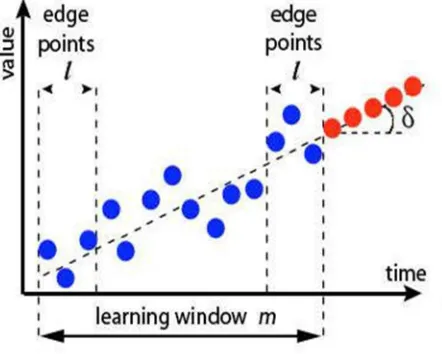
The Derivative Based Prediction (DBP) model is calculated based on a learning window[2]-[3].The learning window, contains two edge points and data points. The two edge points is represented as l and the data points are represented as m. Figure(2) represents the derivative based prediction model. The average values of the edge points in the learning window are connected using the slope

δ.Derivative based prediction name is given to the model since the computation is similar to a computation of a derivative.

Derivative Based Prediction is very efficient computationally by making use of only two edge points.

The algorithm used in DBP is explained in the following, first `m’ consecutive values (the learning window) is taken . Next `l ‘values on right edge and `l’ values on left edge (typically l should be <= m/2) is taken .Subtract average of values from right side edge from the average of those on the left side edge. Divide the resulting number by (m-l) and call it as Derivative . Add the Derivative in the last value of the learning window (the most right side value) to get prediction for m+1 th value.

The (m+2) th value can be obtained by adding the prediction of (m+1)th value to Derivative and so on . For each new value we need to check if the prediction value falls within error tolerance i.e., Is my predicted value within some percentage of actual sensed value. If it is within error tolerance, it is fine we can get the next value by adding continously dervative to this current predicted value . In case predicted value is way too off, we need to regenerate the model i.e., use last m actually sensed values to calculate new derivative using process explained before .

Fig. 2.Derivative Based Prediction Model

99 percentage of transmission of data can be suppressed using derivative based prediction and the quality of the data is also maintained . The life time of the system can be improved to seven fold time by using derivative based prediction.

B. Autoregressive Method (AR)

A random probability distribution or pattern used in statistical calculations in which weighted sum of past values are used to

estimate the future values is known as autoregressive model[9] . Based on the previous input and output Linear prediction formula is used by the autoregressive model to predict the output of the system . An autoregressive model of order p is indicated by the notation AR(p) . AR(P) is given as

(1)

Technology (IJRASET)

©IJRASET: All Rights are Reserved

178

the parameters of the model . Back shift operator B can be used to represent the above equation has the following equation .

(2)

so that, by using the polynomial notation and by moving the summation term to the left side , we have

(3)

To remain wide-sense stationary model Some parameter constraints are necessary. Output of an all-pole infinite impulse response filter whose input is white noise can thus be viewed as

autoregressive model. >1 are not stationary in the AR(1) model process.

To estimate the coefficients, ordinary least squares procedure or method of moments (through Yule–Walker equations)is one of the way.

The AR(p) model is given by the equation

(4)

Between these parameters and the covariance function of the process there is a direct correspondence and to determine the parameters from the autocorrelation function (which is itself obtained from the covariances) this correspondence can be inverted. This is done using the Yule–Walker equations.

(5)

The set of equation above represent the Yule–Walker equations named for Udny Yule and Gilbert Walker .

C. Moving Average Method (Ma)

Creating averages of different subsets of the full dataset in a series, that is used in analysing the data points is known as moving average method[10].For any period of time moving average can be calculated. For forecasting long-term trends moving average calculation is extremely useful . The average calculated for several times for several subsets of data using moving average is exactly the same. “Mean” value of a set of numbers is the representation of the average. For example, if we want a two-year moving average for a data set from 2000, 2001, 2002 and 2003 we would find averages for the subsets 2000/2001, 2001/2002 and 2002/2003. Formula used for forecasting =Sum of last n demand/n. "Moving average" model is a second type of Box-Jenkins model . The concept behind box–jenkins method is quite different but these models look very similar to the AR model. The random errors that occurred in past time periods is related by moving average parameter only to the period t i.e. E(t-1), E(t-2), etc rather than to X(t-1), X(t-2), (Xt-3) as in the autoregressive approaches. Moving average first order term may be written as follows...

X(t)=-B(1)*E(t-1)+E(t) (1)

Where the term B(1) is called an MA of order 1. Model above describes that any given value of the current error term, E(t) to the random error in the previous period, E(t-1), is directly related to X(t). To represent the convention the negative sign is used before the parameters. The moving average models is extended as higher order structures covering moving average lengths this happens in the case of autoregressive models.

Moving-average process of order q is xt if

Xt = Zt + θ1Zt−1 + . . . + θqZt−q (2)

Where Zt = WN(0, σ2 ) and θ1, . . ., θq are constants.

Technology (IJRASET)

©IJRASET: All Rights are Reserved

179

is Xt.

The following equivalent form is another way of representing MA(q)

Xt = θ(B)Zt (3)

The moving average operator is denoted as θ(B). θ(B) defines the values present in the shift operator as

BkZt = Zt−k (4)

Xt is said to be strictly stationary process if Zt is an iid processs. MA(2) process is represented in the below equation

Xt = Zt + θ1Zt−1 + θ2Zt−2 = (1 + θ1B + θ2B2 )Zt. (5)

MA(2) process has zero mean and also it is a combination of a zero mean white noise i.e.,

E Xt = E(Zt + θ1Zt−1 + θ2Zt−2) = 0 (6)

D. Auto Regressive Integrated Moving AVERAGE (ARIMA)

ARIMA forecasting models are based on principles and statistical calculation [7]. A wide spectrum of time series behavior is modeled using arima modeling. AR,MA, ARMA are the three basic model of ARIMA[4] . Applying regular differencing for AR and MA together is defined as ARIMA. Here the integrated and referencing the differencing procedure is indicated as ‘I’. Intervention data, equally spaced univariate time series data, and function data is analysed and forecasted using ARIMA procedure, and intervention data using the AutoRegressive Integrated Moving-Average (ARIMA) or autoregressive moving-average (ARMA) model. The value in a response time series is predicted by the ARIMA model as a linear combination of its past errors (also called shocks or innovations), current and past values of other time series and own past values . Box-Jenkins models is reffered often as ARIMA models. The general transfer function model discussed by Box and Tiao (1975) was employed by the ARIMA procedure. ARIMAX model is sometime referred as ARIMA model, when the other time series are included as input variable by the model.

Four major steps involved in ARIMA modeling are explained below.

1) Model Identification:

a) AR Model: Linear regression model looks like a an AR model except the dependent variable and its independent variables in a regression model are different, whereas the independent variables in an AR model are simply the dependent variable’s time-lagged value , so it is autoregressive. More numbers of autoregressive terms can be included by an AR model .If only one autoregressive term is included by an AR model then it is an AR ( 1 ) model; we can also have AR (2), AR (3), etc and also linear or nonlinear type exist in an AR model.

b) MA Model: Forecast errors produced in the past by weighted moving average of a fixed number is known as MA model. The n weights in a traditional moving average are equal and add up to 1. The MA weights do not sum up and also not equal to 1. Statistical calculation is done in MA by the pattern of the data to determine the number of terms for the model and each term weight. Usally MA carries the most recent values for more than the distant values . One may use the immediate past value or its mean as a forecast for the next future period in a stationary time series.A forecast error is produced in each forecast. A MA model can be developed if the produced error in the past has any pattern. Notice that observed values or not these forecast errors; they are generated values. All MA models are non linear such as MA (1), MA (2),MA (3).

c) ARMA Model: Both AR and MA terms are required by an ARMA model.We must first identify an appropriate model form for the given stationary time series. To identify the given model whether it is an AR or MA or an ARMA we can use the below two

methods

To calculate the partial autocorrelation function and autocorrelation function of the series we use subjective way. To identify the best ARMA model for the data we can use objective methods.

Technology (IJRASET)

©IJRASET: All Rights are Reserved

180

Function (PACF):

In order to use method (1) the ACF and PACF is very important. Calculated from the time series at different lags ACF values fall between -1 and +1 because to determine how far back in time are they correlated and also to measure the significance of correlations between the present observation and the past observations. PACF values are the linear regression coefficients of the time series that use independent variables which is the lagged value . The independent variable coefficient is called first order partial autocorrelation function when only one independent variable of one-period lag is included by the regression. When two period lag is added to the regression as the second term, the second term coefficients is called the second order partial autocorrelation function, etc . If the time series is stationary the values will also fall between -1 and +1 for PACF.

2) Model Estimation: The equation for this model is given below,

y(t) = d + a(1)*y(t-1) + a(2)*y(t-2) – e(t) - c(1)*e(t-1)

N (1)

To produce the forecasts , to fit the model and to optimise the coefficients the above formula is used. Time series analysts found alternative objective methods for identifying ARMA models because of the Box-Jenkins highly subjective nature.

To assist time series analysts penalty function statistics, such as Akaike Information Criterion [AIC] ,Schwarz Criterion [SC] have been used. To factor in model parsimony these statistics all take the form minimizing the sum of squares sum of the residual plus a ‘penalty’ term which incorporates the number of estimated parameter coefficients. The BIC and HQC has the best theoretical properties assuming there is a true ARMA model for the time series.

3) Diagnostic Checking: This part of the diagnostic checking process is useful to know that the model produced reflects the actual time series. To check the validity of ARIMA models Durbin-Watson test is used . The autocorrelation presences in the residuals from a regression analysis is detected by a test statistic known as Durbin–Watson statistic. Durbin-watson statistic is named after Geoffrey Watson and James Durbin.

4) Forcasting: The equation is applied “one step ahead” to get estimate y(t) from observed y(t-1). “kstep- ahead” prediction can also be made by using recursive application of equation .To generate the estimated y at time 2 the observed y at time 1 is used in

recursive application.That estimate is then substituted as y(t-1) to get the estimated y for next t, and same process is repeated so on. The kstep- ahead predictions converge to zero at the end when the kstep-ahead predictions is increased by the prediction horizon.

III. SIMULATION RESULTS

The different data prediction algorithms DBP, AR, MA, and ARIMA are analyzed using the matlab software. The result obtained by using these prediction algorithms on different data set for analysis are shown below. The different data set considered for analysis are

(i)Air temperature 2) AUTOREGRESSIVE ALGORITHM

(ii)Humidity

(iii)Soil temperature (i) AIR TEMPERATURE:

1) DERIVATIVE BASED PREDICTION ALGORITHM

(i) AIR TEMPERATURE:

70

Technology (IJRASET)

©IJRASET: All Rights are Reserved

181

60

Predict ed

50

e(

ce

ls

iu

s)

40

30

20

10 0

5 10 15 20 25

0

Time( hour)

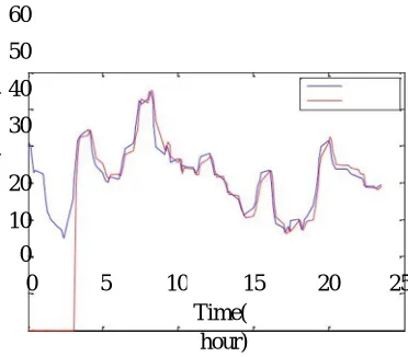
Fig. 3. Graph of Measured Vs Predicted Air Temperature Using DBP.

Figure (3) shows that 144 Air temperature data has been considered for analysis. By implementing DBP algorithm on these data the achieved RMSE is 0.2036(Celsius).

(ii) HUMIDITY:

12 0

Measur ed

Predict ed 10

0

el

si

u

s)

80

60

40

20

0

5 10 15 20 25

0

Time( hour)

Fig. 4. Graph of Measured Vs Predicted Humidity Using DBP.

Figure (4) shows that 144 humidity data has been considered for analysis. By implementing DBP algorithm on these data the achieved RMSE is 0.45889(percentage).

(iii)SOIL TEMPERATURE

Technology (IJRASET)

©IJRASET: All Rights are Reserved

182

45

Measur ed Predict ed 40

ls

ius

)

35 30 25 20

15 10 5 0

5 10 15 20 25

0

Time( hour)

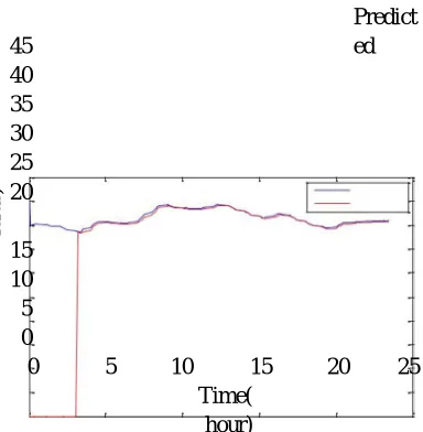
Fig. 5. Graph of Measured Vs Predicted Soil Temperature Using DBP.

Figure (5) shows that 144 soil temperature data has been considered for analysis .By implementing DBP algorithm on these data the achieved RMSE is 0.022779(Celsius).

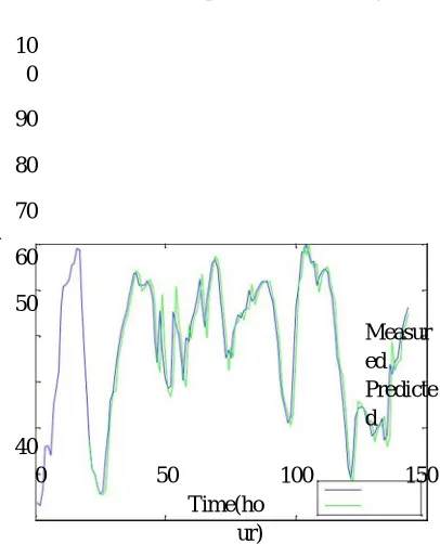
Temperature Forecasting

70 65 60

si

u

s)

55 50 45 40

35 30

25

Measur ed

Predicte d 20

50 100 150

0

Time(h our)

Fig.6. Graph of Measured Vs Predicted Air Temperature Using AR.

Technology (IJRASET)

©IJRASET: All Rights are Reserved

183

(ii) HUMIDITY:

Temperature Forecasting

10 0

90

si

u

s)

80

70

60

50

Measur ed

Predicte d 40

50 100 150

0

Time(ho ur)

Fig. 7. Graph of Measured Vs Predicted Humidity Using AR.

144 humidity data considered for analysis is shown in figure (7). By implementing AR algorithm on these data the achieved RMSE is 0.392188(percentage).

(iii) SOIL TEMPERATURE

Temperature Forecasting

46 45 44

(c

el

si

us

)

43 42 41

40

39 Measur

ed

Predicte d 38

50 100 150

0

Technology (IJRASET)

©IJRASET: All Rights are Reserved

184

Fig. 8. Graph of Measured Vs Predicted Soil Temperature Using AR.

Figure (8) shows that 144 soil temperature data has been considered for analysis. By implementing AR algorithm on these data the achieved RMSE is 0.02282(Celsius).

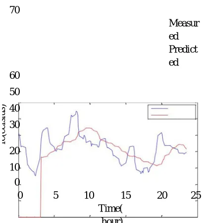
3) MOVING AVERAGE

(i) AIR TEMPERATURE:

70

Measur ed

60

Predict ed

50

re

(c

e

ls

iu

s) 40

30

20

10 0

5 10 15 20 25

0

Time( hour)

Fig. 9. Graph of Measured Vs Predicted Air Temperature Using MA. 4)AUTO REGRESSIVE INTEGRATED MOVING AVERAGE

(i)AIR TEMPERATURE:

Arima Prdictions for AIRTEMP

70

65

Measur ed Predicte d 60

si

u

s)

55 50 45 40

35 30 25 20

50 100 150

Technology (IJRASET)

©IJRASET: All Rights are Reserved

185

Time(ho ur)

Fig. 12. Graph of Measured Vs Predicted Air Temperature Using ARIMA.

144 AIR temperature data considered for analysis is shown in figure(9) . By implementing MA algorithm on these data the achieved RMSE is is 0.716214 (Celsius).

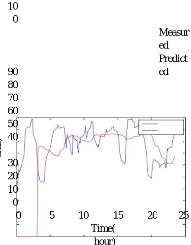
(ii) HUMIDITY:

Figure (12) shows that 144 Air temperature data has been considered for analysis .By implementing ARIMA algorithm on these data the achieved RMSE is 0.081304 (Celsius).

(ii) HUMIDITY:

10 0

90

Measur ed Predict ed 80

si

us

)

70 60 50 40

30 20 10 0

5 10 15 20 25

0

Time( hour)

Fig. 10. Graph of Measured Vs Predicted Humidity Using MA.

Figure (10) shows that 144 humidity data has been considered for analysis . By implementing MA algorithm on these data the achieved RMSE is 1.299505 (percentage).

(iii)SOIL TEMPERATURE

50

45

Measur ed Predict ed 40

Technology (IJRASET)

©IJRASET: All Rights are Reserved

186

30 25 20

15 10 5 0

5 10 15 20 25

0

Time( hour)

Fig. 11. Graph of Measured Vs Predicted Soil Temperature Using MA.

144 soil data considered for analysis is shown in figure(11) .By implementing MA algorithm on these data the achieved RMSE is 0.096878 (Celsius).

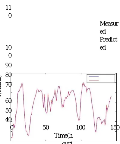
Arima Prdictions for Humidity

11 0

Measur ed

10 0

Predict ed

90

e(

ce

ls

iu

s)

80

70

60

50 40

50 100 150

0

Time(h our)

Fig. 13. Graph of Measured Vs Predicted Humidity Using ARIMA.

144 Humidity data considered for analysis is shown in figure (13) .By implementing ARIMA algorithm on these data the achieved RMSE is 0.086434(percentage).

(iii) SOIL TEMPERATURE

Arima Prdictions for soil

Technology (IJRASET)

©IJRASET: All Rights are Reserved

187

45

Measur ed Predict ed 44

si

us

)

43 42 41 40

39 38 37 36

50 100 150

0

Time(h our)

Fig. 14. Graph of Measured Vs Predicted Soil Temperature Using ARIMA.

Figure (14) shows that 144 Soil temperature data has been considered for analysis .By implementing ARIMA algorithm on these data the achieved RMSE is 0.010276(Celsius).

DATA SET RMSE RMSE RMSE RMSE

USING USING USING USING

DBP MA AR ARIMA

AIR 0.2036 0.716214 0.12607 0.081304

TEMPERATUR E

ROOM 0.45889 1.299505 0.392188 0.086434 TEMPERATUR

E

BASEDON HUMIDITY

SOIL 0.022779 0.096878 0.02282 0.010276 TEMPERATUR

E

TABLE1:PERFORMANCE COMPARISION

Various algorithm has been analysed by applying different data set and their performance comparision is tabulated in the above table1.

IV. CONCLUSION

Technology (IJRASET)

©IJRASET: All Rights are Reserved

188

REFERENCES

[1] Biljana Risteska Stojkoska,Kliment Mahoski “Comparision of different data prediction methods for wireless sensor networks”, 10th Conference for Informatics and Information Technology (CIIT 2013).

[2] U. Raza, A. Camerra, A. Murphy, T. Palpanas, and Picco,“What does model-driven data acquisition really achieve in wireless sensor networks?” in Proc. 10th IEEE Int. Conf. Pervasive Comput.Commun., 2012.

[3] Usman Raza, Alessandro Camerra, Amy L. Murphy, Themis Palpanas, and Gian Pietro Picco “Practical Data Prediction for Real-World Wireless Sensor Networks” IEEE Transactions on Knowledge and Data Engineering, Volume : 27 , issue 8,August 2015.

[4] vJin CUI, Fabrice Valois “Data aggregation in Wireless Sensor Networks: Compressing or Forecasting?”Wireless communication and networking conference (WCNC),IEEE 14.

[5] Rajagopalan, R., & Varshney, P. K. “Data-aggregation techniques in sensor networks: A survey. IEEE Communications Surveys and Tutorials, 4th Quarter, 8(4), 48– 63,2006.

[6] Akkaya, K., Demirbas & Aygun, “The impact of data aggregation on the performance of wireless sensor networks”, Wireless Communications and Mobile Computing, R. S. (2008).

[7] Ayodele A. Adebiyi., Aderemi O. Adewumi ,Charles Ayo “Stock Price Prediction Using the ARIMA Model” 16th International Conference on Computer Modelling and Simulation,2014.

[8] Yao Liang, Yimei Li, “An Efficient and Robust Data Compression Algorithm in Wireless Sensor Networks” IEEE Communications Letters, VOL. 18, NO. 3, March 2014.

[9] Nan Zhao,F. Richard Yu,Hongjian Sun , Hongxi Yin , A. Nallanathan ,Guan Wang “Interference alignment with delayed channel state information and dynamic AR-model channel prediction in wireless networks” Springer Science+Business Media New York 2014.