Munich Personal RePEc Archive
Are we able to capture the EU debt
crisis? Evidence from PIIGGS countries
in panel unit root framework
Baumöhl, Eduard and Výrost, Tomáš and Lyócsa, Štefan
Faculty of Business Economics in Košice, University of Economics in
Bratislava
9 April 2011
Online at
https://mpra.ub.uni-muenchen.de/30334/
Are we able to capture the EU debt crisis?
Evidence from PIIGGS countries in panel unit root framework
Eduard Baumöhl*–Tomáš Výrost –Štefan Lyócsa
Faculty of Business Economics in Košice,
University of Economics in Bratislava, Slovakia
[email protected], [email protected], [email protected]
Abstract
We assess the issue of fiscal sustainability in the selected EU countries. Our sample includes those showing the highest government debts, which are nowadays known under the somewhat degrading acronym – PIIGGS (Portugal, Ireland, Italy, Greece, Great Britain and Spain). Assuming the so-called present value borrowing constraint, stationarity of debts presents a sufficient condition for fiscal sustainability. Utilizing various standard panel unit root tests and the test by Im et al. (2010), we examine this condition on quarterly debt-to-GDP ratios over the period 2000 to 2010. Results provide evidence, that when trend breaks in the series are incorporated, not all of these countries exhibit non-stationarity behavior of their debt-to-GDP ratios.
Key words: Fiscal sustainability, Government debt, Panel unit-root tests JEL classification: E62, C23, H62, H63
Acknowledgement
This paper was supported by grant from Slovak Grant Agency VEGA No. 1/0826/11 and VEGA No. 1/0641/10.
*
1. Introduction
Fiscal sustainability is a key issue for policy makers within the European Monetary Union (EMU henceforth) framework. This topic has been studied quite extensively and is interesting for several reasons: (1) individual fiscal discipline of each EMU member state is relevant to establish the common monetary policy; (2) accumulation of debt in conjunction with subsequent budgetary deficit may invoke an increase of long-term interest rates, which is unfavorable in integrated financial markets where eventually the sovereign debt will be placed scarcely; (3) in compliance with the European Union Treaties, member states adopting the euro have to fulfill the Maastricht convergence criteria (namely in the fiscal area – keeping the level of government debt under the 60 % of GDP of reference value and limiting the deficit at most of 3 % of GDP) and then the Stability and Growth Pact assures, that the fiscal discipline will be monitored henceforward.
We have mentioned three major fields of interest for which the government debt sustainability is relevant. The fourth one stemmed during the recent financial and economic crisis which has resulted in the European sovereign debt crisis, the so-called “2010 Euro Crisis”. Countries showing the highest deficits and debts are nowadays known under the degrading acronym PIIGGS, which stands for Portugal, Ireland, Italy, Greece, Great Britain and Spain. Among other implications, it is unprecedented that the average rate of return from junk bonds is lower (one year yield is 6.372 % as of 11.3.2011 measured by Merrill Lynch High Yield 100 index), than the yield from the government bonds of some EU countries (latest 5 year Portugal emission yields 7.126 %).
The aim of this paper is to assess the government debt sustainability of PIIGGS countries under the present value borrowing constraint. The recent drop in the output of economies, with the long-term increase of debts makes this topic of high interest to policy makers and investors alike. Analysis is conducted by applying standard unit root tests and the test by Im et al. (2010) which allows for a cross-sectional dependence of time series within the panel and break occurrence in both level and trend.
2. Theoretical background and empirical literature overview
A sustainability of public finance is usually presented in the form of present value borrowing constraint (PVBC henceforth). In nominal terms, government budget constraint for one country at time t can be written as1:
t
t t tt r D R D
G 1 1 (1)
where G is the government expenditure, R is the government revenue, D is the government debt and r is the interest rate payable on D. In the absence of money finance, the eventual budget deficit Gt – Rt + rtDt-1 must be financed by an increase of debt Dt – Dt-1.
Equation (1) can be recursively solved for the subsequent periods, whereby inter-temporal budget constraint is formed as:
1 1 1 1 lim 1 s sj t j s t s s j j t s t s t t r D r G R D (2)
We can consider a fiscal policy as sustainable, when the second term from the right-hand side of Equation (2) goes to zero in infinity. The motivation behind stationarity testing lies in the fact, that a stationary Dt+s (around a constant, or a deterministic trend) implies
slower then exponential growth (in the denominator of the right fraction), which would be needed for the debt to be unsustainable.
The PVBC in Equation (1) can also be rewritten using all variables as a percentage of GDP:
tt t t t t t t t t GDP D GDP R GDP g D r GDP G 1 1 1 1 (3)
where the growth rate of GDP is denoted as g. If rt is assumed to be stationary (with
mean r) and g is constant, the PVBC is given by:
0 1 1 1 1 1 lim 1 1 s s s t s s t s t s t r g rg
(4)
where δt = Dt / GDPt; εt = [Gt + (rt –r)Dt-1] / GDPt and ρt = Rt / GDPt. If the last term
in Equation (4) becomes zero (r > g), the fiscal policy will be sustainable and growth of public debt will not become an explosive process. This yields the familiar result that fiscal policy will be sustainable if the present value of the future stream of primary surpluses, as a
1
percentage of GDP, matches the „„inherited‟‟ stock of government debt (Afonso – Rault, 2010)2.
To analyze the fiscal sustainability, two general approaches are applied. The first is to test the government debt for a presence of a unit root3 and the second is to conduct a cointegration analysis between government revenues (R) and expenditures (G)4. When the analyses are conducted on the individual samples of each country, some methodological issues related to the short length of the time series could arise. Such studies therefore often provide mixed results (see, Wilcox, 1989; Uctum – Wickens, 2000 or Bergman, 2001)5. Due to insufficient length of macroeconomic data, several recent empirical papers applied more powerful techniques in a panel framework.
Holmes et al. (2010) analyzed annual budget deficits as a percent of GDP over the sample period 1971 – 2006 for Austria, Belgium, Denmark, Finland, France, Germany, Greece, Ireland, Italy, Netherlands, Spain, Sweden and the United Kingdom. Using Hadri – Rao (2008) test which allows for cross-sectional dependence and for endogenously detected structural breaks, they conclude that EU countries exhibit fiscal stationarity over the full period, even in the subsamples 1971 – 1990 and 1991 – 2006 (pre- and post- Maastricht Treaty). Evidence against the non-stationarity is considered here as support for the strong form of fiscal sustainability insofar as satisfying the PVBC.
Similar conclusions are provided by Afonso – Rault (2010) for the EU-15 countries during the period 1970 – 2006. They found the first difference of stock of government debt to be stationary, using individual LM unit root tests6 (Schmidt – Phillips, 1992; Lee – Strazicich, 2003), panel LM unit root test (Im – Lee, 2001), panel unit root tests with cross-sectional independence (Levin et al., 2002; Im et al., 2003), and panel unit root tests allowing for cross-sectional dependence (Choi, 2006; Moon – Perron, 2004).
In the case of the cointegration tests it is assumed, that R and G are both non-stationary while their first differences are non-stationary. Nevertheless, if one variable is I(0) in levels and the second one is I(1), sustainability is still possible but not observed by
2
For more technical details of PVBC see, e.g., Greiner et al. (2007).
3
For the sake of brevity, we will not distinguish between unit root and stationarity tests (null hypothesis of applied tests will be clearly stated in the results section).
4
According to our knowledge, both procedures to empirical testing of fiscal sustainability were primary applied by Hamilton – Flawin (1986). Some critics of both approaches regarding to PVBC can be found in Bohn (2007).
5
Even though some frequently cited papers (e.g., Ahmed – Rogers, 1995) provide clear results from univariate unit root tests to support the fiscal sustainability.
6
cointegration analysis (for details see Afonso – Rault, 2008). Even when G and R are integrated in different orders, it cannot be clearly stated that there is a sustainability problem (e.g. revenues are systematically above expenditures and budgetary surplus is executed). For this group of empirical studies see, for example, Hamilton – Flawin (1986), Ahmed – Rogers (1995), Prohl – Schneider (2006) or Westerlund – Prohl (2010).
As Afonso – Rault (2010) pointed out; stationarity is a sufficient but not necessary condition for fiscal sustainability. A necessary condition is the existence of a long-run relationship (cointegration) between R and G. Nevertheless, in this paper we will focus on the first approach of testing the fiscal sustainability, i.e. stationarity testing of government debt while several panel unit root test will be applied. It is worth to mention that our sample of data is much more recent and includes the EU debt crisis.
3. Data description and methodology
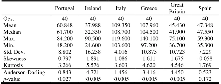
[image:6.595.86.510.497.658.2]To verify the fiscal sustainability of selected EU countries (Portugal, Ireland, Italy, Greece, Great Britain and Spain) we perform various panel unit root tests using debt-to-GDP ratios over the period 2000Q4 – 2010Q3. Some tests require balanced panels, and that is why the time span of our dataset is limited by availability of data which are obtained from the public source – Eurostat. Descriptive statistics and normality tests are presented in the following table.
Table 1: Descriptive statistics and normality test (debt-to-GDP ratios)
Portugal Ireland Italy Greece Great
Britain Spain Obs. 40 40 40 40 40 40 Mean 60.848 37.988 109.350 107.960 45.430 47.348 Median 61.700 32.350 108.700 104.500 41.900 47.550 Max. 84.200 90.500 119.600 140.100 75.100 59.300 Min. 48.200 24.600 103.600 97.200 36.700 35.300 Std. Dev. 8.802 16.258 4.016 10.875 10.723 7.229 Skewness 0.797 1.891 1.086 1.611 1.675 -0.058 Kurtosis 3.266 5.576 3.603 4.620 4.546 1.769 Anderson-Darling 0.843 4.721 1.456 3.416 4.450 0.523
p-value 0.027 <0.005 <0.005 <0.005 <0.005 0.172
Source: Eurostat
It is obvious, that maximum values of debt-to-GDP ratios are affected by recent financial crisis, since the debts tend to increase and moreover, GDPs were decreasing. It can be seen from basic statistics, that Italy and Greece did not kept the level of government debts under the 60 % of GDP within the whole analyzed period. According to above mentioned empirical literature, the stock of debt itself does not provide information about the fiscal sustainability. We can make several conclusions only from descriptive statistics, but our point of interest is whether the unit root tests are able to provide clear results on the matter of debt sustainability of PIIGSS countries.
For this purpose some empirical works utilized univariate unit root tests, which have notoriously low power. This is mostly the case for short span data series and data series with sum of the true autoregressive parameters near, but less than one. If one of the series in the panel framework is stationary, panel tests have higher probability of rejecting the joint null hypothesis of non-stationarity (see, Taylor – Sarno, 1998). Therefore whenever possible, it is currently a standard approach to complement stationarity analysis with panel unit root tests. However, in some tests the joint null hypothesis of a (heterogeneous or homogenous) unit root is not always meaningful. According to alternative hypotheses which claim that some time series are stationary, this only tells the researcher that at least one panel member is stationary, with no information about how many series, or which ones, are stationary (see, Breuer et al., 2002, p. 527).
In the last two decades the research on panel tests has grown rapidly. The distinction between panel tests are made on whether they: assume cross-sectional independence/dependence of the series, assume a common or time series specific data generating process, or allow for structural breaks in the series of the panel. As our samples have only small number of observations, we have not analyzed and assessed univariate stationarity tests. In this paper, we have selected standard, in recent years the probably most widely used tests (Levin et al. (2002) – LLC test; Im et al. (2003) – ISP test; Breitung – Das (2005), Maddala and Wu (1999) –Fisher type χ2 test7, Hadri (2000) – LM test).
For the purposes of our analysis, we also employ a test proposed by Im et al. (2005, 2010), which allows for cross-sectional dependence and structural breaks in the level and trend of the series. As in the previous cases, we again deal with a panel unit root test, which has a potentially greater power when compared to the basic univariate tests. As the choice of
7
Choi (2001) proposed three other Fisher type tests (Z, L* and Pm) in which the power of all the tests increases
available methodologies is large, our choice was motivated by several attractive properties of this particular test.
First, it allows for the presence of breaks both in level and trend. These breaks are not determined endogenously, but have to be identified prior to the unit root testing. This necessity to separate the testing of the unit root hypothesis and break identification may be beneficial, as discussed by Kim – Perron (2009). Particularly, it is possible to avoid the problems with the formulation of the null and alternative hypothesis, such as in the case of the Zivot – Adrews test (1992).
Second, this particular test is based on a statistic with an asymptotic distribution that is free of nuisance parameters, related to the position and the size of the breaks. This property has the advantage that the critical values do not have to be recalculated for the specific breaks found in the data.
In the description of the test used on our sample, we follow the notation and description given by Im et al. (2010; ILT henceforth). We consider a balanced panel dataset with N cross-sectional units and T observations per unit. The vector:
) , , 1 ( it
it t DT
Z (5)
describes the deterministic components in the modeled series, where i denotes the cross-sectional unit (i=1,2,…,N) and t is a time variable (t=1,2,…,T). The variable DTit describing
the break in trend is defined as:
i i
i
b b
b it
t t t t
t t DT
; ; 0
(6)
where
i
b
t is the time index for the occurrence of a break in trend within the series for
cross-sectional unit i. We identify one break for all series in our analysis (see Appendix for detail results). It was possible to allow for breaks in the level of the series, however judging from the data, we considered trend shifts as adequate.
We then follow ILT, by calculating a detrended series
~ ~
~
it it
it y Z
y (7)
where the parameters ~ are obtained from an auxilary regression:
it it it Z u
y
(8)
effect of the constant. ILT suggest that the detrended values should not be used directly, as the distribution of the test statistic would still not be nuissance-free. Instead, they use:
i i i i b it b b it b it t t y t T T t t y t T y ; ~ ; ~ ~* (9)
Using this series, ILT formulate a test equation augmented by cross-sectional averages
of the lagged levels and first differences (yt*1 and yt*) to account for cross-correlation:
it p j j t i ij p j j t ij t t t i i it
it Z y gy h y g y d y u
y
1 , 1 * * * 1 * 1 , ~ ~ (10)
The choice of lag length p was conducted by examining the Schwartz information criterion (BIC) for each series. As the critical values reported by ILT for the final LM statistic assume a common lag choice, we have used lag order of one, the optimal order for the
majority of the series used. The t-statistic (called~i*) for the null hypothesis of i 0 in each
equation can be used to calculate the t-bar statistic:
N i i t 1 * ~ (11)
which in turn can be used to establish the statistic of the LM test having standard normal distribution:
) var( ) ( ) ~ ( * t t E t NLM (12)
The expected value and variance of the t-bar are tabulated by ILT in the Table 3 placed in the appendix of their paper.
4. Empirical findings
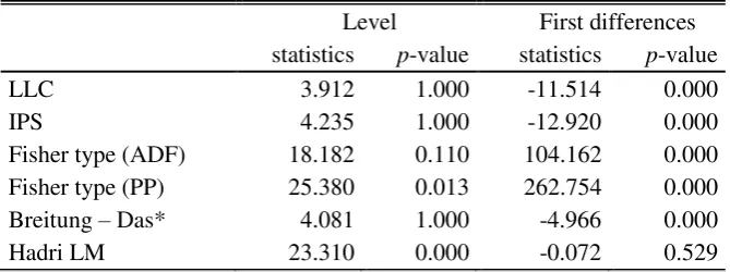
performed on the first differences of the debt-to-GDP ratios. Applying such transformation makes most economic time series stationary (i.e. integrated of order one), which is as well true in our case. The more detailed results are provided in the following table.
Table 2: Results from panel unit root/stationarity tests
Level First differences statistics p-value statistics p-value LLC 3.912 1.000 -11.514 0.000 IPS 4.235 1.000 -12.920 0.000 Fisher type (ADF) 18.182 0.110 104.162 0.000 Fisher type (PP) 25.380 0.013 262.754 0.000 Breitung – Das* 4.081 1.000 -4.966 0.000 Hadri LM 23.310 0.000 -0.072 0.529
Note: trend is included in all tests; * allows for cross-sectional dependence across panel; LLC test H0: all time series have a unit root; H1: all time series are stationary.
IPS test H0: all time series have a unit root; H1: some time series are stationary
Maddala – Wu Fisher type tests H0: all time series have a unit root; H1: some time series are stationary Breitung – Das test H0: all time series have a unit root; H1: all time series are stationary
Hadri LM test H0: all time series are stationary; H1: some time series have a unit root
Since we are dealing with the so-called 2010 Euro Crisis, it is reasonable to assume an occurrence of trend breaks in analyzed series. Over the last two years, due to recent financial and economic crisis, GDPs were decreasing and government debts tend to increase. Both these tendencies have potentially resulted in much higher debt-to-GDP ratios. In the light of these propositions, we continue our analysis by identifying possible breaks in the series.
Rather than testing for the true number of trend breaks, the small sample size of our data, visual inspection and the commonly known facts about the economic crisis in recent years have led us to assume only one break, m = 1. For the date break estimation technique we have followed the commonly used approach of multiple linear regression model, where we have searched for data partitions where the residual sum of squares (RSS) was at a global minimum. For further details of applications see Bai – Perron (1998, 2003) or Zeileis – Kleiber (2005). We have searched for the break date Tj in each of the series by minimizing the
residual sum of squares in the following model:yt 0,j t1,j ut, where j = 1, 2 and
t = Tj-1+1, ….,Tj. The trimming parameter was set only to h = 4 observations from the
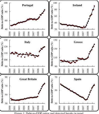
corresponding regime specific estimates of the coefficients are reported in the Appendix. It is also interesting to see, how the size of trend coefficients increased after the identified breaks. The most notable is the case of Ireland, where the coefficient has changed from negative value before the break to highest positive value within the whole sample. These breaks are apparent from graphical visualization of all debt-to-GDP ratios which is presented in the Figure 1.
Figure 1: Debt-to-GDP ratios and detected breaks in trend
Note: The breaks in trends correspond to those obtained by the minimization of RSS, see Appendix for further
details.
As the occurrence of the trend breaks in the data was obvious, we have decided to employ one of the more recent panel unit root tests of Im et al. (2010) which takes into
40 60 80 100
2000 2001 2003 2004 2006 2007 2008 2010
Debt -to -G DP ra tio ( %) Portugal 20 40 60 80 100
2000 2001 2003 2004 2006 2007 2008 2010
Deb t-to -G DP ra tio ( %) Ireland 90 100 110 120 130
2000 2001 2003 2004 2006 2007 2008 2010
Debt -to -G DP ra tio ( %) Italy 90 110 130 150
2000 2001 2003 2004 2006 2007 2008 2010
Deb t-to -G DP ra tio ( %) Greece 30 50 70 90
2000 2001 2003 2004 2006 2007 2008 2010
Debt -to -G DP ra tio (
%) Great Britain
30 50 70
2000 2001 2003 2004 2006 2007 2008 2010
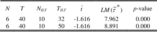
account cross-sectional dependence within the panel and breaks in level and trend as well. The results of the testing procedure on our dataset, together with the parameters tabulated by ILT are shown in the following table.
Table 3: Results from the ILT panel unit root test
N T NILT TILT t LM(~*) p-value
6 40 10 32 -1.616 7.962 0.000 6 40 10 50 -1.616 8.891 0.000
The null hypothesis of the ILT test is that all series in the panel contain unit roots, with the alternative that some of the series are stationary. Our results indicate the rejection of the null hypothesis, that is, we are able to reject the non-stationarity assumption for at least some PIIGGS countries. Thus the sustainability of government debts within the PVBC framework remains partly unresolved for the PIIGGS countries despite of applying one of the latest panel unit root test.
5. Conclusion
In the title of this paper we put a simple question, regarding to ability of standard econometric techniques to capture the recent European sovereign debt crisis. Under the so-called present value borrowing constraint, stationarity of debts is a sufficient condition for fiscal sustainability. Consequently, to resolve this question some standard panel unit root tests has been applied along with one of the latest test proposed by Im et al. (2010).
Appendix
Identified break dates with 95 % confidence intervals
Break date P(2007:Q3 ≤ 2007:Q4 ≤ 2008:Q1) = 95 %
Portugal coefficient variance coefficient variance Intercept 47.98 8.34 -9.42 18.57 Time 0.59 0.10 2.31 0.01
Break date P(2007:Q3 ≤ 2007:Q4 ≤ 2008:Q1) = 95 %
Ireland coefficient variance coefficient variance Intercept 36.58 0.16 -157.80 2.49 Time -0.40 0.00 6.15 0.00
Break date P(2008:Q3 ≤ 2008:Q4 ≤ 2009:Q1) = 95 %
Italy coefficient variance coefficient variance Intercept 110.02 0.35 73.26 11.91 Time -0.13 0.00 1.17 0.01
Break date P(2008:Q1 ≤ 2008:Q2 ≤ 2008:Q3) = 95 %
Greece coefficient variance coefficient variance Intercept 99.35 2.11 -15.03 41.87 Time 0.23 0.01 3.89 0.03
Break date P(2008:Q2 ≤ 2008:Q3 ≤ 2008:Q4) = 95 %
Great Britain coefficient variance coefficient variance Intercept 36.35 0.28 -60.43 99.79 Time 0.26 0.00 3.43 0.07
Break date P(2007:Q4 ≤ 2008:Q1 ≤ 2008:Q2) = 95 %
Literature
[1] Afonso, A. – Rault, Ch. (2008). 3-Step Analysis of Public Finances Sustainability: The Case of the European Union. ECB Working Paper No. 908.
[2] Afonso, A. – Rault, Ch. (2010). What Do We Really Know about Fiscal Sustainability in the EU? A Panel Data Diagnostic. Review of World Economics, 145(4), 731–55. [3] Ahmed, S. – Rogers, J. (1995). Government Budget Deficits and Trade Deficits: Are
Present Value Constraints Satisfied in Long-term Data? Journal of Monetary
Economics, 36(2), 351–74.
[4] Ahmed, S. – Rogers, J. (1995). Government budget deficits and trade deficits. Are present value constraints satisfied in long-term data? Journal of Monetary Economics, 36(2), 351–74.
[5] Bai, J – Perron, P. (1998). Estimating and Testing Linear Models with Multiple Structural Changes. Econometrica, 66(1), 47–48.
[6] Bai, J. – Perron, P. (2003). Computation and Analysis of Multiple Structural Change Models. Journal of Applied Econometrics, 18(1), 1–22.
[7] Bergman, M. (2001). Testing Government Solvency and the No Ponzi Game Condition.
Applied Economics Letters, 8(1), 27–29.
[8] Bohn, H. (2007). Are Stationarity and Cointegration Restrictions Really Necessary for the Intertemporal Budget Constraint? Journal of Monetary Economics, 54(7), 1837–47. [9] Breitung, J. – Das, S. (2005). Panel Unit Root Tests Under Cross Sectional Dependence.
Statistica Neerlandica, 59(4), 414–33.
[10] Breuer, J.B. – McNown, R. – Wallace, M. (2002). Series-specific Unit Root Tests with Panel Data. Oxford Bulletin of Economics and Statistics, 64(5), 527–46.
[11] Choi, I. (2001). Unit Root Tests for Panel Data. Journal of International Money and
Finance, 20(2), 249–72.
[12] Choi, I. (2006). Combination Unit Root Tests for Cross-sectionally Correlated Panels. In: Corbae, D. – Durlauf, S. – Hansen, B. (Eds.), Econometric Theory and Practice:
Frontiers of Analysis and Applied Research, essays in honor of Peter C. B. Phillips.
Cambridge: Cambridge University Press.
[13] Greiner, A. – Köller, U. – Semmler, W. (2007). Debt Sustainability in the European Monetary Union: Theory and Empirical Evidence for Selected Countries. Oxford
[14] Hadri, K. – Rao, Y. (2008). Panel Stationarity Test with Structural Break. Oxford
Bulletin of Economics and Statistics, 70(2), 245–69.
[15] Hadri, K. (2000). Testing for Stationarity in Heterogeneous Panels. The Econometrics
Journal, 3(2), 148–61.
[16] Hamilton, J. – Flavin, M. (1986). On the Limitations of Government Borrowing: A Framework for Empirical Testing. American Economic Review, 76(4), 808–16.
[17] Holmes, M. – Otero, J. – Panagiotidis, T. (2010). Are EU Budget Deficits Stationary?
Empirical Economics, 38(3), 767–78.
[18] Im, K. – Lee, J. – Tieslau, M. (2005). Panel LM Unit-Root Tests with Level Shifts.
Bulletin of Economics and Statistics, 67(3), 393–419
[19] Im, K. – Lee, J. – Tieslau, M. (2010). Stationarity of Inflation: Evidence from Panel Unit Root Tests with Trend Shifts. 20th Annual Meetings of the Midwest Econometrics Group, Oct 1-2, 2010. [online] Available at: <http://apps.olin.wustl.edu/MEG Conference/Files/pdf/2010/70.pdf>
[20] Im, K. – Lee, J. (2001). Panel LM Unit Root Test with Level Shifts. Discussion paper. Department of Economics, University of Central Florida.
[21] Im, K. – Pesaran, M. – Shin, Y. (2003). Testing for Unit Roots in Heterogeneous Panels. Journal of Econometrics, 115(1), 53–74.
[22] Kim, D. – Perron, P. (2009). Unit Root Tests Allowing for a Break in the Trend Function at an Unknown Time Under Both the Null and Alternative Hypothesis.
Journal of Econometrics, 148(1), 1–13.
[23] Lee, J. – Strazicich, M. (2003). Minimum Lagrange Multiplier Unit Root Test with Two Structural Breaks. Review of Economics and Statistics, 85(4), 1082–89.
[24] Levin, A. – Lin, C.F. – Chu, C.S. (2002). Unit Root Tests in Panel Data: Asymptotic and Finite Sample Properties. Journal of Econometrics, 108(1), 1–24.
[25] Llorca, M. – Redzepagic, S. (2008). Debt Sustainability in the EU New Member States: Empirical Evidence from a Panel of Eight Central and East European Countries.
Post-Communist Economies, 20(2), 159–72.
[26] Maddala, G. – Wu, S. (1999). A Comparative Study of Unit Root Tests and a New Simple Test, Oxford Bulletin of Economics and Statistics, 61(0), 631–52.
[27] Moon, H. – Perron, B. (2004). Testing for a Unit Root in Panels with Dynamic Factors.
[28] Prohl, S. – Schneider, F. (2006). Sustainability of Public Debt and Budget Deficit: Panel Cointegration Analysis for the European Union Member Countries. Working Paper No. 0610. Department of Economics, Johannes Kepler University Linz.
[29] Schmidt, P. – Phillips, P. (1992). LM Tests for a Unit Root in the Presence of Deterministic Trends. Oxford Bulletin of Economics and Statistics, 54(3), 257–87. [30] Taylor, M.P. – Sarno, L. (1998). The Behavior of Real Exchange Rates during the
Post-Bretton Woods Period. Journal of International Economics, 46(2), 281–312.
[31] Uctum, M. – Wickens, M. (2000). Debt and Deficit Ceilings, and Sustainability of Fiscal Policies: An Intertemporal Analysis. Oxford Bulletin of Economic Research, 62(2), 197–222.
[32] Westerlund, J. – Prohl, S. (2010). Panel Cointegration Tests of the Sustainability Hypothesis in Rich OECD Countries. Applied Economics, 42(11), 1355–64.
[33] Wilcox, D. (1989). The Sustainability of Government Deficits: Implications of the present-value Borrowing Constraint. Journal of Money Credit and Banking, 21(3), 291– 306.
[34] Yazici, B. – Yolacan, S. (2007). A Comparison of Various Tests of Normality. Journal
of Statistical Computation and Simulation, 77(2), 175–83.
[35] Zeileis, A. – Kleiber, C. (2005). Validating Multiple Structural Change Models – An Extended Case Study. Research Report Series: Department of Statistics and Mathematics Wirtschaftsuniversität Wien, Report 12, January 2005.
[36] Zivot, E. – Andrews, D.W.K. (1992). Further Evidence on the Great Crash, the Oil-Price Shock, and the Unit-Root Hypothesis, Journal of Business and Economic