Enlarged Gradient Observability for Distributed Parabolic Systems: HUM Approach

(1)

ISSN Online: 2153-0661 ISSN Print: 2153-0653

Enlarged Gradient Observability for

Distributed Parabolic Systems: HUM Approach

Hayat Zouiten, Ali Boutoulout, Fatima Zahrae EL Alaoui

TSI Team, MACS Laboratory, Faculty of Sciences, Moulay Ismail University, Meknes, Morocco

Abstract

This paper is focused on studying an important concept of the system analy-sis, which is the regional enlarged observability or constrained observability of the gradient for distributed parabolic systems evolving in the spatial domain

.

Ω_{We will explore an approach based on the Hilbert Uniqueness Method} (HUM), which can reconstruct the initial gradient state between two pre-scribed functions f1 and f2 only in a critical subregion ω of Ω

with-out the knowledge of the state. Finally, the obtained results are illustrated by numerical simulations.

Keywords

Distributed Systems, Parabolic Systems, Regional Enlarged Observability, Gradient Reconstruction, HUM Approach

1. Introduction

Control problem of partial differential equation (PDE) arises in many different contexts and engineering applications. A prototypical problem is that of observability, which is one of the most fundamental concepts in mathematical control theory, and has been the object of various works (see [1], [2], [3]), whose the aim is the possibility to reconstruct the initial state of the distributed system based on partial measurements taken on the system by means of tools called sensors. This concept depends on a very sensitive way of the class of PDE under consideration, in particular, the case of the heat and wave equations.

For distributed parameter systems, the concept of regional observability was introduced by El Jai et al. and interesting results have been obtained, whose target of interest is not fully the geometrical evolution domain Ω, but just in an internal subregion ω_of Ω_(see_[4]_,_[5]_{) or on a part of the boundary} ∂Ω of Ω_(see_[6]_,_[7]_{). Later the notion of regional gradient observability was}

How to cite this paper: Zouiten, H., Bou-toulout, A. and EL Alaoui, F.Z. (2017) En-larged Gradient Observability for Distri-buted Parabolic Systems: HUM Approach.

Intelligent Control and Automation, 8, 15- 28.

https://doi.org/10.4236/ica.2017.81002

Received: November 8, 2016 Accepted: December 27, 2016 Published: December 30, 2016

(2)

developed (see [8]); it concerns the reconstruction of the initial state gradient only in a critical subregion of the system without the knowledge of the state. This concept finds its applications for many real problems. For example, the problem of estimating the energy exchanges between a casting plasma on a plane target which is perpendicular to the direction of the flow sub-diffusion process from measurements carried out by internal thermocouples.

Here we are interested in the concept of the regional enlarged observability of the gradient, which consists in reconstructing the initial gradient state between two prescribed profiles P1 and P2 only in a critical subregion interior of the

evolution domain without the knowledge of the state. The introduction of this concept is motivated by many real problems. This is the case, for example, of the biological treatment of wastewater using a fixed bed bioreactor. The process has to regulate the substrate concentration of the bottom of the reactor between two prescribed levels. This concept was studied using two approaches where the first one is based on subdifferential techniques and the second one uses the Lagrangian multiplier method (see [9], [10]). In this work, we solve this problem using an extension of the Hilbert Uniqueness Method (HUM) developed by Lions (see [11], [12]).

The paper is structured as follows.Section 2 we recall the regional enlarged gradient observability of a linear parabolic system, then we give some definition and properties related to this notion. Section 3 concerns a reconstruction approach using an extension of the Hilbert Uniqueness Method. Section 4 we develop a numerical approach, which is illustrated by simulations that lead to some conjectures.

2. Problem Statement

Let Ω be an open bounded domain in _n₍_n₌_1,2,3_{), with a regular} boundary ∂Ω._For T >0, let’s consider Q= Ω×

[ ]

0,T _and Σ = ∂Ω×

[ ]

0, .T We consider the following system

( )

_{( )}

( )

0

,

, in

,0 in , 0 on ,

y x t

Ay x t Q

t

y x y x

y ξ t ∂ 

=  ∂

 ₌ _Ω



 ₌ _Σ

 

(1)

where A is a second-order linear differential operator with compact resolvent which generates a strongly continuous semi-group

(

S t

( )

)

_t_≥₀ on the Hilbert space _L2

( )

_Ω _._{We assume that} 1

( )

0 0

y ∈H Ω _{is unknown. The observation} space is _₌_L2

(

_{0, ;}_T _q

)

_.

The measurements are obtained by the output function given by

( )

., ,

[ ]

0, ,

z t =Cy t t∈ T ₍₂₎ where C is called the observation operator, linear (possibly unbounded) depending on the structure and the number q of the considered sensors, with dense S-invariant domain

( )

1

( )

0 .

(3)

equations with unbounded observation operator is a system of a linear partial differential equation which describes by pointwise sensors.

Moreover, the system (1) is autonomous the output function can be expressed by

( )

0

( )

0,

[ ]

0, ,

z t =CS t y =K t y t∈ T ₍₃₎ where 1

( )

0

:

K H Ω → is linear operator. To obtain the adjoint operator of

,

K we have

Case 1. C is bounded (e.g. zone sensors) We denote 1

( )

0

: q,

C H Ω → and _C*_{its adjoint. We get that the adjoint}

operator of K can be given by

( )

( ) ( )

* 1

0 *

* * *

0

:

T d .

K H

z S t z t t

→ Ω

→

_∫



Case 2. C is unbounded (e.g. pointwise sensors) In this case, we have

( )

1

( )

0

: q,

C D C ⊆H Ω →_ _with _C*_{denote its adjoint.}

Based on the works (see [13], [14], [15]), to state our results, we have to make the following assumptions:

( )

H1 CS t

( )

can be extended to a bounded linear operator CS t

( )

in

( )

(

1

)

0 , ;

H Ω

 

( )

H2

( )

CS * exists and

( )

CS *=S C* *.

Extend K by K t y

( )

0=CS t y

( )

0, with K∈

(

H01

( )

Ω ,

)

. Then the

adjoint operator of K can be defined as

( )

* * 1

0

* * * *

0

:

T d .

K D K H

z S t C z t t

⊆ → Ω

→

_∫



For ω a subregion of Ω with a positive Lebesgue measure, let χω be the restriction function defined by

( )

(

2

)

(

2

( )

)

:

,

n n

L L

y y y

ω

ω ω

χ ω

χ

Ω →

→ =

with the adjoint χω* given by

* in

0 in \ .

y y ω

ω χ

ω 

=  _Ω

 Let’s consider the operator

( )

(

( )

)

1 2

0

1 :

, , . n

n

H L

y y

x x

∇ Ω → Ω

∂ ∂ 

→ ∇ = _∂ _∂ 

  

Its adjoint is given by

( )

(

)

( )

* 2 1

0 * :

, n

L H

y y v

∇ Ω → Ω

→ ∇ =

(4)

( )

div in

0 on .

v y

v

∆ = − Ω



 ₌ _∂Ω

 (4)

We recall that a sensor is conventionally defined by a couple

(

D f,

)

, where D is its spatial support represented by a nonempty part of Ω_and f is the spatial distribution of the information on the support D. Then the output function (2) can be written in the following form

( )

_D

( ) ( )

, d .

z t =

_∫

y x t f x x ₍₅₎

A sensor may be pointwise (internal or boundary) if D=

{ }

b _with b∈ Ω and f =δ

(

b−. ,

)

_where δ _{is the Dirac mass concentrated in}b, and the sensor is then denoted by

(

b,δ_b

)

._{In this case, the operator}C is unbounded and the output function (2) can be written in the form

( ) ( )

, .

z t = y b t ₍₆₎

We also recall that the system (1) together with the output (2) is said to be exactly (respectively weakly) gradient observable in ω if _Im

(

_K*

)

(

_L2

( )

)

n

ω

χ ∇ = ω

(respectively _Im

(

_K*

)

(

_L2

( )

)

n

ω

χ ∇ = ω ). For more details, we refer the reader to (see [8]).

Let

(

α_i

( )

.

)

_in₌₁_and

(

_{( )}

)

1 . n

i _i

β ₌ _{be two functions defined in}

(

_L2

( )

_ω

)

n_such

that αi

( )

. ≤βi

( )

. a.e. in ω for all 1≤ ≤i n. Throughout the paper we set

( ) ( )

(

)

(

( )

)

( )

{

}

{

2

}

1

. , .

, , n n i . i . i . a.e. in 1, , .

y y L y i n

α β

ω α β ω

 

 

= _ ∈ ≤ ≤ ∀ ∈ _

Definition 1. The system (1) together with the output (2) is said to be

( ) ( )

. , .

α β

 

 -gradient observable in ω if

(

_Im _K*

)

( ) ( )

_{. , .} _.

ω

χ ∇ ∩_α β _≠ ∅

Definition 2. The sensor

(

D f,

)

is said to be _α

( ) ( )

. , .β _ _-gradient strategic in ω if the observed system is _α

( ) ( )

. , .β _-gradient observable in

. ω

Remark 1.

• If the system (1) together with the output (2) is _α

( ) ( )

. , .β __-gradient observable in ω1 then it is α

( ) ( )

. , .β -gradient observable in any subregion

2 1.

ω ⊂ω

• If the system (1) together with the output (2) is exactly gradient observable in ω then it is _α

( ) ( )

. , .β _-gradient observable in ω.

Proposition 1. We have the equivalence between the following statements. 1. The system (1) together with the output (2) is _α

( ) ( )

. , .β _-gradient observable in ω.

2. _{Ker K}

(

* *

)

( ) ( ) { }

_{. , .} _{0 .} ω

χ α β

∇ ∩_ _= Proof. (1) ⇒₍₂₎

(5)

(

*

)

( ) ( )

(

* *

)

( ) ( ) { }

Im χω∇K ∩α . , .β ≠ ∅ ⇒ Ker K∇ χω ∩α . , .β = 0 Suppose that

(

* *

)

( ) ( ) { }

_{. , .} ₀

Ker K∇ χω ∩α β ≠

Let’s consider _{y Ker K}

(

* *

)

( ) ( )

_{. , . ,}

ω

χ α β

∈ ∇ ∩ _ _ such that y≠0. Then

(

* *

)

y Ker K∈ ∇ χω and y∈ α

( ) ( )

. , . .β  We have Ker K

(

* *χω

)

Im

(

χω K*

)

,

⊥

∇ = ∇

thus _y _Im

(

_K*

)

ω

χ ⊥

∈ ∇ such that y≠0. Therefore _y _Im

(

_K*

)

_.

ω

χ

∉ ∇

Then

(

* *

)

( ) ( )

_{. , .}

(

2

( )

)

n_{\ Im}

(

*

)

_.

Ker K∇ χω ∩α β ⊂ L ω χω∇K

Hence

(

*

)

(

2

( )

)

(

* *

)

(

2

( )

)

( ) ( )

Im χω∇K ⊂ L ω n \Ker K∇χω ∪ L ω n\α . ,β . . We have

(

*

)

(

2

( )

)

(

* *

)

Im χω∇K ⊂ L ω n\Ker K∇χω ,

accordingly

(

*

)

(

* *

)

Im χω∇K ∩Ker K∇ χω = ∅,

then

(

*

)

(

*

)

(

)

Im χω K Im χω K Absurd .

⊥

∇ ∩ ∇ = ∅

Since

(

*

)

(

2

( )

)

( ) ( )

Im χω∇K ⊂ L ω n\α . , .β 

we have

(

*

)

( ) ( )

(

)

Im χω∇K ∩α . , .β = ∅ Absurd .

Consequently

(

* *

)

( ) ( ) { }

_{. , .} _{0 .}

Ker K∇χω ∩α β =

(2) ⇒ (1) We shall show that

(

* *

)

( ) ( ) { }

_{. , .} ₀ _Im

(

*

)

( ) ( )

_{. , .}

Ker K∇ χω ∩α β = ⇒ χω∇K ∩α β ≠ ∅

Suppose that

(

* *

)

( ) ( ) { }

_{. , .} _{0 .}

Ker K∇χω ∩α β = Let’s consider

(

* *

)

( ) ( )

_{. , . ,}

y Ker K∈ ∇χω ∩ α β  then

(

* *

)

_and

( ) ( )

_{. , . , such that} _0.

y Ker K∈ ∇ χω y∈α β  y=

(6)

(

* *

)

_Im

(

*

)

_{, so} _Im

(

*

)

_{such that} _0,

Ker K χω χω K y χω K y

⊥ ⊥

∇ = ∇ ∈ ∇ =

hence

(

*

)

( ) ( )

Im and . , . .

y∈ χω∇K y∈ α β 

Thus

(

*

)

( ) ( )

Im χω∇K ∩α . , .β ≠ ∅,

which shows that the system (1) together with the output (2) is _α

( ) ( )

. , .β __- gradient observable in ω.

3. HUM Approach

In this section, we present an approach that allows the reconstruction of the initial gradient state in _α

( ) ( )

. , . .β _ The approach constitutes an extension of the Hilbert Uniqueness Method developed by Lions (see [11]) to the case of regional enlarged observability of the gradient. Let the initial state gradient decomposed in the following form

( ) ( )

( )

(

)

( ) ( )

1 0

0 ₂ ₂

0

in . , .

in n\ . , .

y y

y L

α β

 _ _

 = 

Ω  

 _ _



(7)

In the sequel our object is the reconstruction of the component y10 in

( ) ( )

. , . , α β

 

  let G be defined by

( )

(

)

(

( )

)

( ) ( )

{

2 2

}

{

1

( )

}

0

0 in \ . , . .

n n

G= g∈ L Ω g= L Ω _α β _ ∩ ∇f f H∈ Ω ₍₈₎

For 1

( )

0 H0 ,

φ ∈ Ω _{we consider the system}

( )

_{( )}

( )

0

,

, in

,0 in , 0 on

x t

A x t Q

t

x x

t

φ

φ φ

φ ξ ∂ 

=

 _∂

 ₌ _Ω

 

= Σ

 

(9)

which admits a unique solution 2

(

1

( )

)

(

[ ]

)

0

0, ; 0,

L T H C T

φ∈ Ω ∩ Ω× (see [16]). Let us go further in the state reconstruction by considering various types of sensors.

3.1. Pointwise Sensors

In this case, the output function is given by

( )

, , 0,

[ ]

z t = y b t t∈ T ₍₁₀₎ where b∈ Ω denote the given location of the sensor.

For φ0∈G, there exists a unique φ ∈0 H01

( )

Ω such that φ0 = ∇φ0. Then

we consider the semi-norm on G be defined by

( )

1

2 ₂

0 0 ₀

1 , d ,

n T

G _k

k

b t t

x φ

φ φ

=

 _ _∂ _ 

 

=  _∂ 

   



∫

∑



(7)

where φ the solution of (9). We consider the following retrograde system

( )

_{( )}

_{( ) (}

₎

(

)

( )

* 1 * ,

, , in

, 0 in ,

0 on ,

n

k k

A x t

A x t b t x b Q

t x

x T t

ψ _ψ φ _δ

ψ ψ ξ ν =  ∂ ∂ − = + − ∂ ∂ 

 ₌ _Ω

 ∂

 ₌ _Σ

 ∂ 

∑

(12)

which admits a unique solution 2

(

1

( )

)

0

0, ;

L T H

ψ∈ Ω _(see_[16]_). Let the operator Λ be defined by

( )

(

)

* 0 0 : 0 G G φ φ Λ →

→ Λ = Ψ

  _ (13)

where * ω ω χ χ =

 and Ψ

( )

0 =

(

ψ

( )

0 , ,_ψ

( )

0 .

)

Let’s consider the system

( )

_{( )}

_{( ) (}

₎

(

)

( )

* 1 * ,

, , in

, 0 in ,

0 on ,

n

k k

A

z x t _{A z x t} y _{b t} _{x b} _Q

t x

z x T

z t δ ξ ν =  ∂ ∂ − = + − ∂ ∂ 

 ₌ _Ω

 ∂

 ₌ _Σ

 ∂ 

∑

(14)

If φ0 is chosen such that z

( )

0 =ψ

( )

0 in ω, then the system (14) could

be seen as an adjoint of the system (1) and our problem of the enlarged gradient observability is to solve the equation

( )

(

)

0 Z 0 ,

φ

Λ =  (15)

where Z

( )

0 =

(

z

( )

0 , , 0 , z

( )

)

with z is the solution of the system (14). Proposition 2. If the system (1) together with the output (2) is _α

( ) ( )

. , .β __- gradient observable in ω, then the equation (15) admits a unique solution

0 G,

φ ∈ _{which coincides with the initial gradient state} y1₀ to be observed in

( ) ( )

. , . .

α β

 

 

Proof. 1. Firstly, we show that if the system (1) together with the output (2) is

( ) ( )

. , .

α β

 

 -gradient observable in ω, then (11) defines a norm on G. Let’s consider φ0∈G, we have

( )

[ ]

0 0

1 1

0 eit , n i 0 a.e. in 0, .

i

G i k k

b T

x

λ φ

φ ∞ φ ϕ

= = ∂ = ⇒ = ∂

∑

 Then

( )

0 1

, n i 0, .

i k k b i x ϕ φ ϕ = ∂ = ∀ ∂

∑

Since the observed system is _α

( ) ( )

. , .β _-gradient observable in ω, we

obtain

( )

1 0, .

(8)

Then φ ϕ0, _i =0, hence φ =0 0. Consequently φ0=0. Thus (11) is a norm. 2. Now let us prove that (15) has a unique solution. Equation (15) admits a unique solution if the operator Λ is an isomorphism.

Indeed, multiplying (12) by k x

φ ∂

∂ and integrating the result over Q, we obtain

( )

( ) (

)

( ) * 2 2 2 1 , , , , , , , , , .

k L Q k L Q

n

l

k l L Q

x t x t x t A x t

x t x

x t b t x b

x x

φ ψ φ _ψ

φ φ _δ

= ∂ ∂ ∂ = − ∂ ∂ ∂ ∂ ∂ − − ∂

∑

∂ which gives

( ) ( )

( )

2 2 0 * 0 2 1 , , , , , ,

, , , , , d .

T

k L k L Q

n T

l

k L Q k l

x t x t x t x t

x x t

x t A x t b t b t t

x x x

φ _ψ φ _ψ

φ _ψ φ φ

Ω =  _∂  _{∂ ∂}_ _   − _ _ ∂ ∂ ∂       ∂ ∂ ∂ = − − ∂

∫

∂

∑

∂

With the initial condition, we have

( ) ( )

( )

( ) ( )

( )

2 2 * 0 2 1

,0 , ,0 , , ,

, , , , , d

k L k L Q

n T

l

k L Q k l

x x A x t x t

x x

x t A x t b t b t t

x x x

φ _ψ φ _ψ

φ _ψ φ φ

Ω = ∂ ₌ ∂ ∂ ∂ ∂ ∂ ∂ − − ∂

∫

∂

∑

∂

Using the Green formula, we obtain

( ) ( )

( )

0

2 1

,0 , ,0 T , n , d .

l

k L k l

x x b t b t t

x x x

φ _ψ φ φ

= Ω ∂ ₌ ∂ ∂ ∂

∫

∂

∑

∂ Hence

( ) ( )

( )

0 2

1 1 1

,0 , ,0 , , d .

n n _T n

k k L k k l l

x x b t b t t

x x x

φ _ψ φ φ

= _Ω = =

∂ ₌ ∂ ∂

∂ ∂ ∂

∑

∫

∑

Thus

( )

2

0 0 ₀

1

, T n , d .

l l

b t t

x

φ φ φ

=

 ∂ 

Λ _{= } _

∂ 

∑



∫

  Then 2

0, 0 0 .

G φ Λφ = φ

We deduce that Λ is an isomorphism, consequently the equation (15) has a unique solution φ0∈G which corresponds to the initial state observed in

( ) ( )

. , . . α β

 

 

3.2. Zonal Sensors

(9)

The system is augmented with the output function

( )

_D

( ) ( )

, d .

z t =

_∫

y x t f x x (16) In this case, we consider the system (9), G is given by (8), and we define a semi-norm on G by

( )

( ) 1 2 ₂ 0 ₀ 2

1 , d .

n T

G k k L D

t f t

x φ φ =  _ _∂ _   _ _  =  _ ∂ _     

∑

∫

 ₍₁₇₎

With the system

( )

_{( )}

( )

(

)

( )

* 2 1 * ,

, , in

, 0 in ,

0

n

D

k k L D

A x t

A x t t f f x Q

t x

x T t

ψ _ψ φ _χ

ψ ψ ξ ν = ∂ ∂ − = + ∂ ∂ = Ω ∂ = ∂

∑

on ,

       _Σ   (18)

we introduce the operator

( )

(

)

* 0 0 : 0 , G G φ φ Λ →

→ Λ = Ψ

  _ (19)

where * ω ω χ χ =

 and Ψ

( )

0 =

(

ψ

( )

0 , , 0 ._ψ

( )

)

Let’s consider the system

( )

_{( )}

( )

(

)

( )

* 2 1 * ,

, , in

, 0 in ,

0

n

D

k k L D

A

z x t _{A z x t} y _{t f} _{f x} _Q

t x

z x T

z t χ ξ ν = ∂ ∂ − = + ∂ ∂ = Ω ∂ = ∂

∑

on .

       _Σ   (20)

If φ0 is chosen such that z

( )

0 =ψ

( )

0 in ω, then the system (20) can be

seen as an adjoint of the system (1) and our problem of the enlarged gradient observability is to solve the equation

( )

(

)

0 Z 0 ,

φ

Λ =  (21) where Z

( )

0 =

(

z

( )

0 , , 0 , z

( )

)

with z the solution of the system (20).

Proposition 3. If the system (1) together with the output (2) is _α

( ) ( )

. , .β __- gradient observable in ω, then the equation (21) has a unique solution φ ∈0 G,

which coincides with the initial gradient state 1 0

y observed in _α

( ) ( )

. , . .β _ Proof. The proof is similar to the pointwise case.

4. Numerical Approach

We consider the system (1) observed by a pointwise sensor located in b∈ Ω. In the previous section, it was shown that the regional enlarged observability of the initial gradient state in _α

( ) ( )

. , .β __{is equivalent, in all cases, to solving the} equation

( )

(

)

0 Z 0 ,

φ

(10)

The numerical approximation of (22) is realized when one can have a basis

( )

ϕ_{i i}

∈ of

(

( )

)

2 n

L Ω _{and the idea is to calculate the components}Λ_ij_{of the} operator Λ.

Then we approximate the solution of (22) by the linear system

0

1 for 1, , ,

N

ij j i

j Z i N

φ =

Λ = =

∑

 _ ₍₂₃₎

where N is the order of approximation and Zi are the components of

( )

(

Z 0

)



(

i=1, ,_ N

)

_{in the basis considered.}

Let

( )

ϕ_{i i}_∈_ be a complete set of the eigenfunctions of the operator A in

( )

1

0 ,

H Ω _{which is orthonormal in}_L2

( )

_Ω _._{We also consider a basis of}

( )

(

_L2 _Ω

)

n_{denoted by}

( )

_.

i i

ϕ

∈ Then the components Λij are the solutions of

the following equation, for a pointwise sensor

( )

, 1 1 1

, 1

, , , , , ,

e 1

, 1, , .

k k l l

ij

i j

i j n n

T

k l n

k l

m p

k l m p

x x x x

b b

x x

k l

λ λ

ϕ ϕ ϕ ϕ

ϕ ϕ ϕ ϕ λ λ ∞ = + =  ∂ ∂  ∂ ∂ 

 _ _ × _ _ Λ

∂ ∂ ∂ ∂  _ _ _ _   ₋ ∂ ∂ = + ∂ ∂   ₌ _∞ 

∑

   (24)

In the case of a zonal sensor

(

D f,

)

, we obtain

( )

( ) ( )

, 1 1 1

, 1 2 2

,..., , ,..., ,

e 1 _, _, _,

, 1, , .

k k l l

ij

i j

i j n n

T

k l n

k l

m p

k l m _{L D} p _{L D}

x x x x

f f

x x

k l

λ λ

ϕ ϕ ϕ ϕ

φ ϕ ϕ ϕ λ λ ∞ = + =  ∂ ∂  ∂ ∂ 

 _ _ × _ _ Λ

∂ ∂ ∂ ∂  _ _ _ _  ∂ ∂  ₋ = ×  ₊ _∂ _∂   ₌ _∞   

∑

 (25)

Then, we have the following algorithm : Algorithm.

Step 1: The subregion ω,_{the location of the sensor b.}

Choose the function y0∈ α

( ) ( )

. , . .β 

Threshold accuracy ε.

Step 2: Repeat

 Solve the system (9) to obtain φ.  Solve the system (14) to obtain z.

 Solve the equation (23) to obtain φ0.

Until y0−φ0 2

_{( )}

_L2_{( )}_ω n <ε.

Step 3: The solution φ0 corresponds to the initial gradient state to be

ob-served in _α

( ) ( )

. , . .β _

5. Simulation Results

(11)

location.

Let’s consider the following one-dimensional system in Ω =

[ ]

0,1 excited by a pointwise sensor

( )

_{[ ]}

( )

[ ]

2

0

, ,

0.01 in 0,

,0 in 0, 1, 0 in 0, ,

y x t y x t

T

t x

y x y x

y t y t T

∂ ∂

= Ω×



∂ ∂

 ₌ _Ω



 ₌ ₌

 

(26)

augmented with the output function

( ) ( )

, , .

z t =y b t b∈ Ω₍₂₇₎ The initial gradient state to be reconstructed is

( )

(

)(

)

0 2 1 1 .

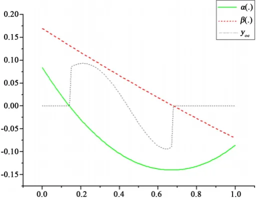
y x =x x− x− We take b=0.18 and T=2, with

( )

1 1 2 and

( )

2 1 1 .

7 2 3 3 30 4

x x x x x x

α =_ − _ − _ β =_ − _ − _

     

[image:11.595.228.522.216.542.2] [image:11.595.245.504.356.556.2]

Applying the previous algorithm, we obtain the following results: •_For ω=

]

0.15,0.70

[

Figure 1. The estimated initial gradient state y0e.

Figure 1 shows that the initial gradient state estimated y0e is between α

( )

. and β

( )

. in ω=

]

0.15,0.70 ,

[

_{then the location of the sensor is} _α

( ) ( )

. , .β _- gradient strategic in ω.

The initial gradient state yoe is estimated with a reconstruction error

2 3

0 oe 2.84 10

y ₋y ₌ _× −

•_{If the sensor is located in b = 0.32, we obtain the} Figure 2.

(12)

[image:12.595.261.488.70.242.2]

Figure 2. The estimated initial gradient state y0e.

[image:12.595.211.540.334.454.2]

Here numerically we study the dependence of the gradient reconstruction error with respect to the subregion area of ω. We have the following Table 1.

Table 1. Relation between the subregion and the reconstruction error.

Subregion The reconstruction error

]0.15, 0.85[ _{3.68 10}_× −1

]0.2, 0.7[ _{1.11 10}_× −1

]0.35, 0.65[ _{6.03 10}_× −2

]0.10, 0.35[ _{2.44 10}_× −2

]0.20, 0.30[ _{6.19 10}_× −3

Table 1 shows how the reconstruction error grows with respect to the subregion area.

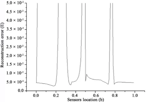
[image:12.595.253.496.544.713.2]

The following simulation results show the evolution of the observed gradient error with respect to the sensor location.

(13)

Figure 3 shows how the worst locations of the sensor correspond to a great error, which corresponds to the non-strategic sensor location.

6. Conclusion

In this work, we have considered the problem of regional enlarged observability of the gradient for parabolic linear systems. We explored an approach that leads to the reconstruction of the initial gradient state between two prescribed functions. The obtained results were applied to the head equation in a one- dimen- sional case and illustrated by numerical example and simulations. Future works aim to extend this notion in Γ_{a part of the boundary}∂Ω_{of the} system evolution domain Ω.

Acknowledgements

This work has been carried out with a grant from Hassan II Academy of Sciences and Technology.

References

[1] EL Jai, A. and Pritchard, A.J. (1988) Sensors and Actuators in Distributed Systems Analysis. Ellis Horwood Series in Applied Mathematics, John Wiley & Sons, Hobo-ken, New Jersey.

[2] Curtain, R.F. and Pritchard, A.J. (1978) Infinite Dimensional Linear Systems Theory. Lecture Notes in Control and Information Sciences, 8, Springer, New York. https://doi.org/10.1007/BFb0006761

[3] Curtain, R.F. and Zwart, H. (1995)An Introduction to Infinite Dimensional Linear Systems Theory. Texts in Applied Mathematics, 21, Springer Verlag, New York.

https://doi.org/10.1007/978-1-4612-4224-6

[4] Amouroux, M., EL Jai, A. and Zerrik, E. (1994) Regional Observability of Distri-buted Systems. International Journal of Systems Science, 25, 301-313.

https://doi.org/10.1080/00207729408928961

[5] EL Jai, A., Simon, M.C. and Zerrik, E. (1993) Regional Observability and Sensors Structures. Sensors and Actuators Journal, 39, 95-102.

https://doi.org/10.1016/0924-4247(93)80204-T

[6] Zerrik, E., Badraoui, L. and El Jai, A. (1999) Sensors and Regional Boundary State Reconstruction of Parabolic Systems. Sensors and Actuators Journal, 75, 102-117. https://doi.org/10.1016/S0924-4247(98)00293-3

[7] Zerrik, E., Bourray, H. and Boutoulout, A. (2002) Regional Boundary Observability: A Numerical Approach.International Journal of Applied Mathematics and

Com-puter Science, 12, 143-151.

[8] Zerrik, E. and Bourray, H. (2003)Gradient Observability for Diffusion Systems. Int.

Journal of Applied Mathematics and Computing, 13, 139-150.

[9] Boutoulout, A., Bourray, H. and Baddi, M. (2011) Constrained Observability for Parabolic Systems. International Journal of Mathematical Analysis, 5, 1695-1710. [10] Boutoulout, A., Bourray, H. and Baddi, M. (2011) Regional Observability with

Con-straints of the Gradient.International Journal of Pure and Applied Mathematical, 73, 235-253.

(14)

[12] Lions, J.L. (1989) Sur la contrôlabilité exacte élargie. Progress in Nonlinear

Diffe-rential Equations and Their Applications, 1, 703-727.

[13] Balakrichnan, A. (1976) Applied Function Analysis. Springer-Verlag, Berlin. [14] Pritchard, A.J. and Wirth, A. (1978) Unbounded Control and Observation Systems

and Their Duality. SIAM Journal on Control and Optimization, 16, 535-545. https://doi.org/10.1137/0316036

[15] Reed, M. and Simon, B. (1972) Methods of Mathematical Physics 1: Functional Analysis. Academic Press, New York.

[16] Lions, J.L. and Magenes, E. (1968) Problèmes aux limites non homogènes et appli-cations. Vol. 1 and 2, Dunod, Paris.

Submit or recommend next manuscript to SCIRP and we will provide best service for you:

Accepting pre-submission inquiries through Email, Facebook, LinkedIn, Twitter, etc. A wide selection of journals (inclusive of 9 subjects, more than 200 journals)

Providing 24-hour high-quality service User-friendly online submission system Fair and swift peer-review system

Efficient typesetting and proofreading procedure

Display of the result of downloads and visits, as well as the number of cited articles Maximum dissemination of your research work