Munich Personal RePEc Archive
Quantitative and credit easing policies at
the zero lower bound on the nominal
interest rate
Dai, Meixing
BETA, University of Strasbourg, France
2011
Online at
https://mpra.ub.uni-muenchen.de/28129/
Quantitative and credit easing policies at the zero lower bound on
the nominal interest rate
Meixing DAI*
Abstract: Using a New-Keynesian model extended to include credit, money and reserve markets, we examine the dynamics of inflation and output gap under some monetary policy options adopted when the economy is hit by large negative real, financial and monetary shocks. Relaxing the assumption that market interest rates are perfectly controlled by the central bank using the funds rate operating procedure, we have shown that the equilibrium at the zero lower bound on the nominal discount rate is stable (or cyclically stable, depending on monetary and financial parameters) and constitutes a liquidity trap, making the central bank’s communication skills useless in the crisis management. While the quantitative easing policy allows attenuating the effects of crisis, it is not always sufficient to restore the normal equilibrium. Nevertheless, quantitative and credit easing policies coupled with the zero discount rate policy could stabilize the economy and make central bank’s communication potentially credible during the crisis.
Key words: Zero lower bound (ZLB) on the nominal interest rate, zero interest rate policy, liquidity trap, quantitative easing policy, credit easing policy, dynamic stability.
JEL Classification: E43, E44, E51, E52, E58.
_________________________
1. Introduction
During the recent global financial and economic crisis, we have witnessed a certain number of
most prominent central banks in the world, e.g. the Federal Reserve, the European central bank
(ECB), the Bank of England and the Bank of Japan, have brought down the discount and funds
rates to a level near to zero, and massively inject the central-bank liquidity into the money and
credit markets under what is called quantitative and credit easing policies.
The monetary policy experience of Japan during the 1990s and 2000s has stimulated a vivid
interest among economists on the “liquidity trap” in the sense of Keynes, i.e. whatever is the
quantity of central-bank liquidity injected into the money market, it is absorbed without a
decrease of the nominal money-market interest rate notably because the latter has encountered the
zero lower bound (ZLB). The interest has grown larger after the burst of the Internet bubble in
2000 because many economists doubt that the USA could enter a deflation crisis.
Various proposals have been advanced to make monetary policy effective in the event of the
ZLB on nominal interest rates. One widely shared belief among economists is that pre-emptive
monetary easing is important to minimize the likelihood that interest rates will fall to zero. Studies
on the issue of pre-emptive monetary easing include, among others, Orphanides and Wieland
(2000), Reifschneider and Williams (2000), Kato and Nishiyama (2005), Adam and Billi (2006,
2007), Nakov (2008), and Oda and Nagahata (2008).1 For Benhabib et al. (2002), a route to
avoiding self-fulfilling liquidity traps is to modify monetary policy, by switching from Taylor rule
to a money growth rate target letting interest rates be market determined, when the economy
seems to be headed toward a low-inflation spiral. This change of policy regime may be effective
when fiscal policy is not Ricardian. Buiter and Panigirtzoglou (2003) and Buiter (2009) have
proposed the use of Gesell taxes on monetary balances, which can be interpreted as a negative
interest rate on money, as a way to avoid liquidity traps.2 This point of view is contested by
Benhabib et al. (2002) who argue that if a liquidity trap is understood as a situation where the
opportunity cost of holding money (instead of bonds) becomes zero, a Gesell tax clearly does not
eliminate it but simply pushes the nominal interest rate on bonds at which it occurs below zero.
Another important consensus among economists is that, when nominal interest rates have
fallen to zero, “expectations management” which acts on the formation of private-sector
expectations about future monetary policy is important. A relatively large literature about
“expectations management” is developed since the work of Krugman (1998), who argues that,
even when the nominal interest rate hits the ZLB, the central bank could still stimulate the current
level of output by raising expectations of future inflation.3 Most economists working on the issue
of interest rate ZLB share this point of view and suggest that the Bank of Japan commits to
policies that would raise future inflation. However, raising inflation expectations and committing
to reducing the policy interest rates in the future are not separate issues since it is by committing
to lower future policy rates that the central bank affects future inflation at the ZLB (Eggertsson
and Woodford, 2003, 2004; Jung et al., 2005; Adam and Billi, 2006, 2007; Nakajima, 2008;
Walsh, 2009). Three alternative policy proposals involving a yen depreciation are advanced. The
first calls for an aggressive base money expansion when the nominal rate reaches zero
(Orphanides and Wieland, 2000). The second suggests that the central bank switches to an
exchange rate-based Taylor rule when the ZLB is encountered, with the exchange rate adjusted in
response to inflation and output gap (McCallum, 2000, 2001). The last proposal, due to Svensson
(2001, 2003), calls for a depreciation followed by an exchange rate peg and an announced
price-level target. However, these proposals have limited utility if several large economies
simultaneously enter into a liquidity trap. Altering the composition of assets on the central bank’s
2 Buiter (2009) has made two other proposals, i.e. (1) abolishing currency; (2) decoupling the numéraire from the currency/medium of exchange/means of payment and introducing an exchange rate between the numéraire and the currency. The exchange rate is set over time to achieve a forward discount or expected depreciation of the currency vis-à-vis the numéraire when the nominal interest rate in terms of the numéraire is set at a negative level for monetary policy purposes.
balance sheet offers another potential lever for monetary policy while the effectiveness of such
policies is a contentious issue (Bernanke and Reinhart, 2004). Auerbach and Obstfeld (2005) have
shown that an open-market purchase of government debt can counteract deflationary price
tendencies when the ZLB is encountered. Furthermore, the central bank can also alter monetary
policy by changing the size of its balance sheet through buying or selling securities to affect the
overall supply of reserves and the money stock. Therefore, even if the overnight interest rate
becomes pinned at zero, the central bank can still expand the quantity of reserves beyond what is
required to hold the overnight rate at zero or a very low level. Such policy, commonly referred to
as “quantitative easing” is experimented firstly in Japan and currently in the United-States, the
euro zone and the United-Kingdom.
There is some evidence that quantitative easing can stimulate the economy even when interest
rates are near zero. The quantitative easing policy that leads to an expansion of the money supply
at the ZLB will affect the economy as long as the rise in the money supply is expected to persist
(Sellon, 2003). According to Spiegel (2006), in the case of Japan, the real effects of quantitative
easing appear to be principally associated with some measurable declines in longer-term interest
rates.4 These have been associated both with changes in agents’ expectations of future interest rate
levels and with purchases of “nonstandard” assets, such as longer-term government bonds. Since
quantitative easing and other unconventional monetary policies often occurred simultaneously, it
is difficult to discriminate between them.
The Fed has gone much further down the path of quantitative easing. In particular, it focuses
on expanding the asset side of its balance sheet in order to lower interest rates on the credit
markets. In such a policy, compared to what the Fed has traditionally done through the
open-market operations or discount, the range of assets accepted is much broader, they have much
longer maturities and the number of financial institutions that have access to the central-bank
liquidity has been significantly increased following a relaxation of criteria and a change in the
status of some institutions. The Bank of England, the ECB to a lesser extent, has followed the
practice of the Fed. Even though market observers initially use the term “quantitative easing”, the
Fed Chairman Ben Bernanke (2009) has preferred to use the term “credit easing”. The difference
between quantitative easing and credit easing does not reflect any doctrinal disagreement with the
Japanese approach, but rather the differences in financial and economic conditions between the
two episodes. The new term allows the Fed Chairman to better communicate with the public on
unconventional policy measures and to make a difference with a monetary policy involving only
the injection of central-bank liquidity through the increase of banking reserves.5 Policies which go
beyond the quantitative easing policy such as buying private-sector credit instruments or lending
by the central bank have been previously discussed in some studies (Clouse et al., 2003; Sellon,
2003). However, such policies are not yet discussed in a theoretical framework which clearly
distinguishes quantitative and credit easing policies.
We remark that using similar framework as the literature on inflation targeting and interest
rate rules, theoretical studies about the ZLB on the nominal interest rate do not make explicit the
links between monetary policy and extremely negative financial and monetary shocks and hence
are not wholly satisfactory for studying the underlying transmission mechanism of the effects of
zero interest rate, and quantitative and credit easing policies. Discussions about the quantitative
easing policy are made generally without using models except Auerbach and Obstfeld (2005),
while the latter use a framework which cannot be used to discuss how quantitative and credit
easing policies could interact. Furthermore, most theoretical frameworks do not explicitly
consider the operating procedure of the central bank by not distinguishing the overnight, longer
term interbank and credit market interest rates. When discussing about the ZLB on the nominal
interest rate, most economists talk in effect about the funds rate targeted by the central bank. The
ZLB on the funds rate becomes a problem because we are concerned with the market interest rates
which can be higher if market operators perceive that the monetary policy of lowering funds rate
is not sufficient to restore the economic growth and the confidence on the financial markets.
Hence, it is very important to make the distinction between the funds rate and other market
interest rates.
This paper provides a framework where several policies options, such as zero interest rate
policy, and quantitative and credit easing policies used in the current financial and economic
crisis, could be simultaneously examined. We extend a New Keynesian framework (Clarida et al.,
1999) to a model of policy analysis with credit, money and reserve markets where the funds rate
operating procedure is explicitly integrated. It offers a more realistic view about how the interest
rate policy is first put in place through the targeting of very short-run interest rate, contrary to the
existing monetary policy literature which assumes that the central bank directly controls the
interest rate affecting the aggregate demand. Thus, it allows understanding why these policies
become suddenly necessary under extreme financial stress. It clarifies the links between the
inflation-targeting regime and these policies when important financial and monetary shocks hit the
economy. Our objective is to examine the dynamics of inflation and output gap when some or all
of these policy options are adopted and how these variables will behave when a particular exit
strategy is adopted.
The remainder of the paper is structured as follows. The next section presents the New
Keynesian model extended to include credit, money and reserve markets. The third section
presents the dynamics of inflation rate and output gap under the standard inflation-targeting
regime. The fourth section examines the dynamic stability of the economy when it is hit by large
persistent real, financial and monetary shocks such that the ZLB on the nominal discount rate is
attained. In the fifth section, we examine the inflation and output-gap dynamics under quantitative
2. The model
The supply and demand sides of the economy are described by a stylized new-Keynesian model:
t t t t
t β π λx επ
π = Ε +1+ + , with 0<β <1, λ >0, (1)
xt t
t ct t
t
t x i
x =Ε +1−ϕ( −Επ +1)+ε , with ϕ >0, (2)
where πt (≡ pt− pt−1) denotes the rate of inflation, pt the (log) general price level, xt the output
gap (i.e., the log deviation of output from its flexible-price level), itc the nominal credit market
interest rate at which non-financial private sector can borrow from banks.
Equation (1) represents the New-Keynesian Phillips curve, where the inflation rate is related
to the expected future inflation rate (Εtπt+1) and current marginal cost, which is affected by the
output gap. The inflation shock, επt, is due to productivity disturbances.
Equation (2) is the expectational IS curve which relates the current output gap to the expected
future output gap (Εtxt+1) and the real credit market interest rate. The latter is defined as the
difference between the nominal credit-market interest rate ict and the expected future rate of
inflation, i.e. (ict −Εtπt+1).
We assume that the individual saver can save at ict if she directly buys bonds emitted by
firms, which offer a rate of return equal to ict. Furthermore, for simplicity, savers are assumed to
save in a deposit account bearing no interests at banks and hence the intertemporal arbitrage
between present consumption and saving depends only on ict. The aggregate demand shock, εxt,
reflects either productivity disturbances which affect the flexible-price level of output or,
equivalently, changes in the natural real interest rate. Without explicitly introducing asset prices,
we admit that εxt could also include wealth shocks affecting the aggregate demand.
The money market equilibrium condition is given by
lt mt t t
t p lx l i
m − = 1 − 2 +ε , with l1 ,l2 >0, (3)
where imt is the nominal interest rate determined on the money market at which the banks can
The money supply is endogenous but it is imperfectly elastic as the banking system will increase
or decrease the internal money taking account of nominal interest rate and will not always satisfy
the demand of this money (or credit) if it is expected to be unwarranted by collaterals. Similarly,
the central bank provides a limited quantity of central-bank liquidity on the reserve market to a
limited number of banks by accepting certain categories of assets as collaterals. Instead, if the
central bank desires, control can be exercised over a narrow monetary aggregate such as base
money (including reserves and currency), and its variations are then associated with these in
broader measures of money supply.
The link between the total money supply and the base money is modeled as follows:
t mt t t b hi
m = + 1 +ω , h1>0 . (4)
where bt is the base money in log terms, and money multiplier (mt−bt in log terms) is assumed
to be an increasing function of the nominal money-market interest rate, and ωt is a
money-multiplier disturbance. The money supply function is similar to that adopted by Modigliani et al.
(1970), and McCallum and Hoehn (1983).
We assume that the central bank indirectly targets money and credit market interest rates
through the funds rate targeting procedure. Under this operating procedure, the central bank
indirectly targets ict or imt, longer term interest rates, by targeting in the first place the funds rate
(ift), a very short-run or overnight interest rate. More precisely, the central bank controls the
discount rate, idt, and conducts open market operations in order to affect the supply of reserves in
the banking system to target the funds rate. We assume that the access to the central-bank
liquidity at the discount window is submitted to nonprice rationing, so that ift ≠idt.6Similarly, we
assume that the access to inside liquidity created within the banking and financial system here is
subject to non-price rationing so that we generally have imt ≠ift ≠idt.
Adopting a simplified description of the reserve market to establish the link between the base
money bt and the discount rate idt, the money supply under the funds rate targeting procedure
can be rewritten as (Appendix A)
mt dt mt t
t b hi hi
m =~ + 1 − 2 +ε , h1,h2>0, (5)
where b~t represents the currency in log terms but could also include the component of the
reserves that the central bank can discretionarily control by adjusting the ratio of obligatory
reserves, and εmt represents shocks affecting the base money under the funds rate targeting
procedure as well as these affecting the monetary multiplier. According to (5), the central bank,
by controlling the discount rate, has not a strict control over the money supply since the latter is
affected by the money-market interest rate and a random shock. However, in order to modify the
behaviors of private agents and their inflation expectations, control can be exercised by the central
bank over b~t, a component of base money which do not depend on the discount rate. The
equilibrium condition on the money market (3) is rewritten as
lt mt t t mt dt mt
t hi h i p lx l i
b~ + 1 − 2 +ε − = 1 − 2 +ε . (6)
In the following, we assume that h1−h2+l2>0. This is justified on the ground that the
supply of liquidity by the banking sector is most likely determined by the difference (imt −idt), i.e.
the net gain obtained from providing more liquidity while refinancing it at the discount rate. Thus,
an increase of equal amount in idt and imt will not (or modestly) affect the money supply but will
significantly reduce the money demand, ceteris paribus.
The model is completed by a credit market equilibrium condition in the spirit of Bernanke and
Blinder (1988):
ct ct t ct
mt f i jx j i
i
f + = − +ε
− 1 2 1 2 , with f1,f2, j1, j2>0, (7)
where εct denotes a random shock that includes both credit supply and credit demand shocks.
Equation (7) gives the credit-market clearing condition and it allows determining ict for given
mt
with ict and it is an increasing function of output gap xt due to transactions demand for credit,
which might arise, for example, from working capital or liquidity considerations. We admit that
0
2 2 1− f − j <
f , i.e. an increase of identical amount in imt and ict will leave the credit supply
stable or decreasing less (because the lending margin in absolute terms is unchanged and only the
margin in relative terms is reduced) than the credit demand.
Some modifications relative to the model of Bernanke and Blinder have been introduced.
Public bonds are not included in the present model since its rate of return could stay relatively
stable in the event of important negative financial shocks affecting private sectors. The private
bonds are assumed to be a perfect substitute to bank lending. Another modification consists to
assume that the longer term money-market interest rate imt, instead of long term public bonds,
affects both the demand and supply of liquidity on the money market. For simplicity, we have
assumed that imt does not affect consumption and investment decisions. Despite these
simplifications, by giving a special attention to reserve, money and credit markets, we can quite
realistically expose how the central bank’s interest rate policy makes its way into the economy.
Such a framework is more adapted for examining how the inflation expectations behave when the
ZLB on the nominal interest rate is encountered.
When the central bank sets idt, it must recursively determine the target of idt using equations
(6)-(7) once the target of credit market interest rate is known. Thus, given that the money-market
equilibrium condition (6) determines the value for idt in order to attain the target of other interest
rates, it follows that the money supply cannot be endogenously determined using (6) as it is
usually assumed in the inflation targeting literature (Woodford, 1998; King, 2000).
In the inflation-targeting literature, it is assumed that the money supply automatically adjusts
to the money demand so that the money market can be ignored without serious consequences. In
this model, by assuming that market interest rates and discount rate are distinct, the central bank
will not always be able to control the market interest rates without manipulating the money
adjust to satisfy the money demand except when the central bank maintains the risk premium on
the money-market interest rate over the discount rate, ρmt =imt −idt, at a fixed level. This opens
the door to quantitative or/and credit easing policies, considered as useful tools to target market
interest rates in critical situations, i.e. when the discount rate cannot be decreased anymore due to
the ZLB on the nominal interest rate.
The model is closed with the specification of central bank’s objective function, which
translates the behavior of the target variables into a welfare measure to guide the policy choice.
We assume that this objective function is over the target variables x t and πt, and takes the form:
∑
∞= + +
− + Ε
=
0
2 2
] ) (
[ 2
1
i
T i t i t i t
CB x
L β α π π , (10)
where the parameter α is the relative weight on output deviations. The central bank’s loss
depends on output gap variability around of zero and inflation variability around of its constant
target πT which can be zero or positive. Since xt is the output gap, the loss function takes
potential output as the target. The strategy of flexible inflation targeting is implemented through
an optimal nominal interest rate rule, which is deduced from the optimal inflation-targeting rule of
the central bank which acts to minimize fluctuations of output gap and inflation rate around their
respective target under discretion.
The time sequence of events is as follows: 1) Workers form inflation expectations and
negotiate wages taking account of all available information about the economy. 2) Shocks realize.
3) The central bank sets the discount rate following an optimal interest rate rule. 4) Firms decide
their production and prices.
The minimization of loss function (10) subject to the Phillips curve (1) leads to the following
targeting rules in the sense of Svensson (2002):
)
( t T
t
x π π
α
λ −
−
= , (11)
)
( 1
1
T t t t
tx α π π
λ Ε −
− =
Equations (1)-(2) and targeting rules (11)-(12) allow defining the following instrument rule in
the sense of Svensson (2002):
xt t T t t T ct i ε ϕ ε λ α ϕ λ π λ α αϕ λ π λ α αϕ λ α αβ λ π 1 ) ( ) ( ) ( ) (
1 2 2
3 1 2 2 + + + + + Ε + − − +
= + , (13)
The optimal target of credit-market interest rate, ictT, implied by the minimization of central
bank’s loss function, must react positively to the expected future rate of inflation if
0 ) (
)
(α+λ2 +λ αβ−α−λ2 >
αϕ . It reacts positively to a variation in πT, and shocks εtx and εtπ.
The credit-market interest rate is indirectly controlled by the central bank through the funds rate
targeting procedure. The latter affects then the longer term money-market interest rate before
affecting the credit-market interest rate.
Using (7) and (13), we deduce that the optimal target of money-market interest rate imtT :
) ( 1 1 ) ( ) ( ) ( ) ( 1 1 1 2 2 3 1 2 2 1 2 2 ct t i xt t T t t T
mt jx
f f j f i T ct ε ε ϕ ε λ α ϕ λ π λ α αϕ λ π λ α αϕ λ α αβ λ
π − +
+ + + + + Ε + − − + + = +
, (14)
which shows that imtT is positively related to T ct
i and it depends on the structural parameters of the
credit market and shocks affecting the latter.
Using (6) and (14), we obtain the optimal target of discount rate
). ~ ( 1 ) ( 1 1 ) ( ) ( ) ( ) ( 1 ) ~ ( 1 2 2 1 1 1 2 2 3 1 2 2 1 2 2 2 2 1 2 2 1 2 2 1 lt mt t t t ct t xt t T t t lt mt t t t T mt T dt p b h x h l x j f f j f h l h p b h x h l i h l h i ε ε ε ε ϕ ε λ α ϕ λ π λ α αϕ λ π λ α αϕ λ α αβ λ ε ε π − + − + − + − + + + + + Ε + − − + + + = − + − + − + = + (15)
Equation (15) allows then determining the target for average funds rate (see Appendix A).
In normal situation, when the financial markets function smoothly, the ZLB on the nominal
discount rate will not be hit. Assume that the central bank sets the discount rate to attain the other
interest rate targets under the funds rate operating procedure. Using (13)-(15), the equilibrium risk
), ( 1 1 ) ( ) ( ) ( ) ( 1 1 1 2 2 3 1 2 2 1 2 2 1 ct t x t t T t t T mt T ct ct x j f f j f f i i ε ε ϕ ε λ α ϕ λ π λ α αϕ λ π λ α αϕ λ α αβ λ ρ
π − +
+ + + + + Ε + − − + − − = − = + ). ~ ( 1 ) ( 1 1 ) ( ) ( ) ( ) ( 1 2 2 1 1 1 2 2 3 1 2 2 1 2 2 2 2 1 2 lt mt t t t ct t x t t T t t T dt T mt mt p b h x h l x j f f j f h l h h i i ε ε ε ε ϕ ε λ α ϕ λ π λ α αϕ λ π λ α αϕ λ α αβ λ ρ π − + − + − + − + + + + + Ε + − − + + − − = − = +
The equilibrium risk premiums depend on the parameters characterizing the structure of goods,
credit, money and reserve markets, inflation expectations, inflation target, output gap, as well as
shocks affecting these markets. They could be kept at relatively low level when the economy is in
expansion but could be enlarged to a high level, incompatible with the optimal interest rate policy
defined under the inflation-targeting regime.
Equations (13)-(15) capture well the complexity of indirect market interest rate targeting
through the funds rate operating procedure. The transmission mechanism is imperfectly
observable by the central bank since it could be hit by numerous unanticipated shocks affecting
the goods, credit, money and reserve markets. Furthermore, shocks affecting the interest rate
policy could also interfere with the transmission mechanism. In some circumstances, negative
disturbances in financial and corporate sectors can create dislocation on financial markets and
enlarge the difference between the discount rate, and the money- and credit-market interest rates
such that the discount and funds rates hit the ZLB while the market interest rates are still too high
for the economy to recover from a severe depression.
3. Inflation and output dynamics in the benchmark model
In the inflation-targeting literature, it is a usual practice to assume that all interest rates are equal.
Therefore, a funds rate targeting procedure is equivalent to the one directly targeting the interest
rate which directly affects the aggregate demand. This assumption could be justified if all
financial assets are perfect substitutes, all financial and monetary markets function perfectly and
Under this kind of assumptions, the model is reduced to (1)-(2). Subject to these two
equations, the central bank minimizes the loss function (10). This leads to the targeting rules
(11)-(12) and the optimal credit-market interest rate rule (13). If the central bank sets the credit market
interest rate following (13), the targeting rules (11)-(12) will be verified. Thus, the difference
equation for the inflation rate is deduced using (1) and (11):
t T
t t
t αβπ β επ
λ π α λ β
π 1(1 ) 1
2 2
1= + − −
Ε + . (16)
The eigenvalue of the difference equation (16) is greater than unity. Consequently, as there is one
forward-looking variable, i.e. Εtπt+1, the equilibrium is stable. The dynamics of output gap is
determined by that of inflation rate according to the targeting rule (12). We remark that the
inflation dynamics is governed by a very simple mechanism and depends uniquely on parameters
characterizing the Phillips curve and central bank preferences.
4. Inflation dynamics when the ZLB on the discount rate is hit
We observe that the ZLB on the nominal discount and funds interest rates are hit in Japan during
the 2000 and now in USA during the current financial crisis. One common point between these
two circumstances is that both countries are exposed to colossal speculative bubbles on several
asset markets. Therefore, the ZLB on the nominal interest rate cannot be appropriately examined
if such shocks can not be taken into account in the model. This is the case in the standard
New-Keynesian model where the ZLB on the nominal discount and funds interest rates is often
confused with the ZLB on the credit-market interest rate. The later has neither been effectively
observed in Japan nor in the USA or any other country. The present model introduces the money,
credit and reserve markets and hence allows to consider the effects due to the burst of the bubbles
in the prices of real and financial assets through the shocks affecting different markets. It is to
notice that real, financial and monetary shocks that lead the economy into a liquidity trap and the
period of sustained rapid economic expansion and the burst of great speculative asset price
bubbles formed during the period.
During the last two decades, using an interest rate policy, central banks in many countries
have achieved the “great moderation” characterized by moderate and stable inflation rate and less
fluctuation of output growth around its potential. A benign macroeconomic environment of great
moderation could encourage financial agents to abandon their prudent approach of investing,
lending and other financing decisions which balance macroeconomic and idiosyncratic risks, and
to progressively espouse exuberant approaches (Carney, 2009). Thus, they take the maximum risk
exposure compatible with the existing regulations, thinking that they all have the chance of
quitting the sinking Titanic ship before the others or that the monetary and fiscal authorities will
save them.
The asset bubbles created under this state of spirit could favour the success of monetary and
fiscal policies. Therefore, policymakers might seek to create bubbles and might not want to take
account of the potential damages induced by their burst because such damages will only
materialize in the future and create difficulties for future policymakers. When the bubbles attain
the extreme limit, menacing hence the central bank’s principal objectives of price stability and
output stabilization, they will be indirectly pricked by policymakers through creating monetary or
fiscal conditions unfavourable for them to continue to grow rapidly. Their burst generates great
financial and monetary as well as real shocks because a large number of agents have been
excessively involved, often with large leverage based on overpriced collateral. The failure of
some great financial institutions becomes a dilemma for the monetary and fiscal authorities.
Avoiding any potential bankruptcy among these institutions envoys a bad message according to
which the speculative feast could continue. On the opposite, not bailing out them could induce
financial panics, amplifying hence the shocks generated by the burst of large asset bubbles.
When such bubbles are pricked, to avoid dramatic consequences on the real economy (i.e.
the case of Japan, the zero nominal discount rate is not sufficient to avoid the deflation and it does
not provide a sufficient stimulus for the economy. Therefore, the question is under what
conditions the deflation (or, on the contrary, the hyperinflation) can be avoided and how will
behave the expected inflation rate and output gap once such a policy is implemented.
The ZLB on the nominal interest rate is hit when the target of discount rate determined by
(15) is less than or equal to zero, i.e. idtT ≤0. The zero interest rate policy corresponds to a
suboptimal equilibrium if setting the discount rate at zero cannot bring the credit-market interest
rate to a level which is optimal for the central bank because the optimal target of discount rate is
smaller than zero. To make the monetary policy effective, large negative shocks on goods, credit,
money and reserve markets imply a need for simultaneously implementing zero discount rate, and
quantitative and credit easing policies.
When shocks affecting money and credit markets generate major dislocations on goods and
labor markets, the dynamics of inflation expectations will be greatly modified. The expectations
of future inflation and output gap will be determined quite differently compared to these under a
normally functioning inflation-targeting regime where they, always independent of financial and
monetary shocks, will be determined by the central bank’s targets except when inflation shocks
are persistent. When the ZLB on the nominal discount rate is hit, the optimal targeting rules in the
sense of Svensson (2002) will not be verified. The current and expected inflation rates and output
gaps will depend on the functioning of credit and money markets because the latter determine the
credit-market interest rate which directly affects the aggregate demand. Therefore, shocks
affecting credit, money and reserve markets will be transmitted through this channel to the
inflation rate and output gap. This mechanism is unconceivable in standard New-Keynesian
models where credit, money and reserve markets are absent and where the ZLB on the nominal
discount rate is confounded with that on the credit-market interest rate.
Knowing that, when the ZLB on the nominal discount rate is hit, the equilibrium conditions
of current and future inflation rates and output gaps, the central bank and private agents who want
to form good inflation expectations cannot neglect the developments on these markets,
particularly, when the functioning of credit and money markets is such that any inadequate
monetary policy response to these shocks can put the economy either on diverging inflationary or
deflationary paths for a long time.
The model is solved by determining recursively the money-market interest rate imt using (6)
for idt =0 and then the nominal credit-market interest rate ict using (7) and finally substituting
the solution of ict into the IS equation (2). The resulting equation and the Phillips curve (1) allow
solving for equilibrium values of expected and current inflation rates and output gaps and
determining if a crisis equilibrium is stable or not.
Using (6), the money-market interest rate is expressed by:
) ~
( 1
1 2
1
mt lt t t t
mt p b lx
l h
i − + +ε −ε
+
= . (17)
In a liquidity trap, εlt is likely to be important and εmt likely to be small. Even though the output
gap could be negative, its impact could be insignificant for bringing down the nominal
money-market interest rate, a median term rate, to zero.
Using (7) and (17), the credit-market interest rate is given as
+ + − + + − +
+
= t t t lt mt t ct
ct p b lx jx
l h
f j f
i 1 ε ε 1 ε
2 1
1
2 2
) ~
( 1
. (18)
During a period where the economy is affected by large negative financial shocks, the credit
demand is likely to decrease but the credit supply could decrease further as banks become more
prudent or impose more restrictive conditions on credit distribution, so that εct is likely to be
positive and could be more than compensating the effects of negative output gap on the
Substituting ict determined by (18) into (2), and taking account of (1), we obtain the inflation
rate and output gap as function of expected inflation rate, output gap, current price level, current
stock of currency and different shocks:
) (
1
1 t t t
t
tπ = β π −λx −επ
Ε + , (19)
ε ϕ ϕ ϕ β λϕ π β ϕ t t t t t t t l h j f b p f x l h j f l f j f j
x +Σ
+ + − + + + + + + + + − = Ε + ) )( ( ) ~ ( ) )( ( 1 2 1 2 2 1 2 1 2 2 1 1 2 2 1
1 , (20)
where Σεt = f +jfϕh+l εlt −εmt +βϕεπt+ f ϕ+j εct−εxt 2 2 2 1 2 2
1 ( )
) )(
( . Since pt = pt−1(1+πt), the system
constituted of (19)-(20) has two forward-looking variables, Etxt+1 and Etπt+1, and one
predetermined variable, pt−1. Equation (20) could be rewritten as:
. ) )( ( ~ ) ( ) )( ( 1 ) )( ( ) ( 2 1 2 2 1 1 2 1 2 2 1 1 2 2 1 2 1 2 2 1 1 1 ε ϕ ϕ ϕ β λϕ ϕπ π π β ϕ t t t t t t t t t t l h j f b f x x l h j f l f j f j l h j f f x x ∆Σ + + + ∆ − − + + + + + + + + + + − − = − Ε − − + (21)
The private sector is assumed to form rational inflation expectations conditional on
information available at t. The equilibrium value of πt−1, xt−1, πt, xt, Etπt+1, and Etxt+1 can be
solved in accordance with the method of undetermined coefficients (McCallum, 1983). Since
these solutions are quite cumbersome and they are not central to the dynamic analysis of inflation
and output gap, they are not given in this paper. We pay instead our attention to the
complementary solutions.
Denote the eigenvalues of the difference equations (19) and (21) by e. We can show that they
must satisfy the following relation (Appendix B):
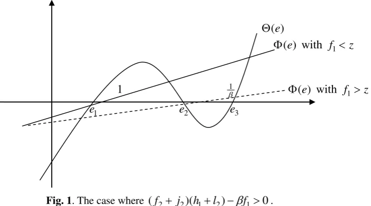
The nature of the dynamic system will depend on the roots of the polynomial
) ( ) ( )
(e e e
F =Θ −Φ . Since the exact solutions of these roots will not be interpretable due to their
complexity, to study the magnitude of these roots, it turns out convenient to use a mixture of
graphical and analytical techniques. Therefore, to find e solving F(e)=0 is equivalent to find e
solving the equation Θ(e)=Φ(e). The left hand of this equation, Θ(e), is a cubic function and
the right hand of this equation Φ(e) linear function. Assume that the financial system is
sufficiently developed, algebraic analysis combined with graphical method shows that two kinds
of dynamics can be distinguished (Appendix C). 7
In the event where f1< (f2+j2β)(h1+l2), the credit supply is insufficiently elastic with regard to
money-market interest rate. In this case, there is one positive eigenvalue which is smaller than
unity but two eigenvalues greater than unity. Given that the dynamic system has two
forward-looking variables and one predetermined variable, the crisis equilibrium is stable.
If f1> (f2+j2β)(h1+l2), i.e. the credit supply is sufficiently elastic with regard to the
money-market interest rate, there is one positive eigenvalue which is smaller than unity. There are two
complex eigenvalues with a positive real part greater than unity. Hence, the crisis equilibrium is
cyclically stable.
In both cases considered above, the crisis equilibrium is stable. Consequently, it could form a
liquidity trap so that a temporary injection of liquidity will not be able to modify the expectations
about future inflation and output gap and hence the crisis equilibrium. As the crisis equilibrium is
stable, it is impossible to pull the economy out of financial and economic crisis by talking
optimistically to financial market operators and the general public because there does not exist a
diverging trajectory leading the economy out of the crisis equilibrium.
Since the crisis equilibrium is a liquidity trap, the central bank must react quickly and
vigorously to avoid this equilibrium to be anchored in private expectations by using policy
measures which could counterbalance the effects of violent financial and monetary shocks.
Several possibilities offered to the central bank. One is to act on the monetary market through
massively increasing the reserves or/and currency. Another is to increase the credit supply by
buying private bonds to fully compensate the effects of real, financial and monetary shocks on the
credit-market interest rate.
The actions on the money market may not be enough if the decrease in money-market interest
rate is not (or only very partially) transmitted to the credit market, i.e. if f1 tends to be very small.
In this case, there might need a very great increase in the reserves and/or currency, which could be
incompatible with the mandate of the central bank and could disturb the market expectations,
leading hence to criticism of the central banker.
5. Quantitative and credit easing policies and dynamic stability
In many industrial countries, the burst of large bubbles in real and financial asset prices formed
during the decade of “great moderation” could be a long process and could affect the economic
equilibrium during a long period. To avoid that their burst leads to developments similar to these
observed in Japan during the decades 1990 and 2000, where the prices of real state and stocks are
still largely lower than the highest levels attained at the end of 1989, appropriate policy responses
are necessary to answer to the waves of real, financial and monetary shocks linked to such a burst.
Absorbing large negative disturbances on the goods market may require a low credit-market
interest rate which may not be within the reach of the central bank when the financial and
monetary markets are also affected by large negative disturbances and the ZLB on the nominal
discount and funds interest rates is encountered. By manipulating only the discount rate and
targeting funds rate through open market operations to indirectly affect the lending interest rates,
the central bank has no credible instrument of anchoring the inflation expectations besides the
cheap talk about its firm intention to attain its inflation target and to stabilize the economy. The
inflation rate and output gap are stabilized, and is converging to the crisis equilibrium. If this is
the case, non-orthodox monetary policy, such as quantitative easing policy, must be used to ease
the tension on the money market. Furthermore, the credit easing policy could be needed in order
to ease the conditions on the credit market, through for example strengthening banks’ balance
sheet and/or buying private debts on the credit market by the central bank or Treasury.
These two monetary policies could be clearly distinguished in our framework. Due to the ZLB
on the nominal discount rate as well as the malfunctioning of money and credit markets, the zero
interest rate policy does not allow the realization of optimal money- and credit-market interest
rates. In this case, the effective money- and credit-market interest rates determined by the
equilibrium conditions on money and credit markets will be higher than their respective optimal
target given by (14) and (13). If no measure is taken to directly affect the equilibrium conditions
on the money and credit markets, the targeting rules (11)-(12) will not be effective.
In the following, we first analyze the inflation and output gap dynamics under the quantitative
easing policy as practiced by the Bank of Japan. Then, we turn to analyze the dynamics of these
variables under a combination of quantitative and credit easing policies as in the case of the Fed,
the Bank of England or the ECB.
5.1. Quantitative easing policy
The quantitative easing policy defined in the sense of Ben Bernanke is only directed to the money
market. It consists to inject an important quantity of reserve which is greater than what is
necessary to keep the funds interest rate at zero. By targeting the liquidity in the banking and
financial system, the quantitative easing policy is used to induce an increase in the supply on the
credit markets through the reduction of the money-market interest rate. The abundance of liquidity
in the banking system is such that banks will not try to retain it by fear of its penury. This allows
stimulating interbank lending and could bring down the money- and credit- market interest rates.
level which is compatible with the normal equilibrium in the absence of financial and monetary
shocks. Denote by qe the quantity of base monetary in the form of reserves injected by the central
bank into the banking system, the equilibrium condition on the money market (6) is rewritten as:
lt mt t t mt dt mt t
e b hi hi p lx l i
q +~+ 1 − 2 +ε − = 1 − 2 +ε . (23)
By targeting the liquidity on the money market, the central banks can reduce the effects of
excessively adverse money supply and demand shocks which drive the money-market interest rate
to a too high level incompatible with the realization of inflation and output-gap targets. For
0
=
dt
i and qe >0, (23) gives the money-market interest rate as:
) ~
( 1
1 2
1
mt lt t t t e
mt q b p lx
l h
i − − + + +ε −ε
+
= . (24)
Consider in the following three scenarios.
Positive optimal target of money-market interest rate
If the target of money-market interest rate given by (14) is positive, i.e. imtT ≥0, the central bank
can use the quantitative easing policy to achieve the objectives of macroeconomic stabilization
and to ensure the dynamic stability of inflation expectations as under the standard
inflation-targeting regime by setting qe to ensure that imt =imtT . If this is the case, the quantitative easing
policy is fully efficient in the sense that the targeting rules (11)-(12) are verified and the effects of
shocks affecting aggregate demand, and credit, money and reserve markets are fully
counterbalanced. The inflation and output dynamics is similar to that in the benchmark case
corresponding to the standard inflation-targeting regime described in section 3. In this scenario,
the economy is confronted a financial and economic crisis which does not constitute a liquidity
trap.
If shocks affecting negatively the aggregate demand, and money and credit supplies, and
positively the demand for liquidity are extremely large and persistent, the central bank may not be
able to counterbalance them. In effect, responding to such large shocks by injecting very large
quantity of central-bank liquidity into the banking and financial sectors could lead to the criticism
of the central bank for sowing seeds for future asset price bubbles and moral hazards in these
sectors. This could induce the central bank, instead of restoring the optimal equilibrium, to
conduct an incomplete quantitative easing policy in the sense that the realized money market
interest rate given by (24) is higher than its target level, i.e. imt >iTmt. Given imt determined by
(24), the nominal credit-market interest rate is
+ + − + + + − − + +
= e t t t lt mt t ct
ct q b p lx jx
l h
f j
f
i 1 ε ε 1 ε
2 1 1 2 2 1 ) ~ ( ) ( ) ( 1
, (25)
which is higher than the optimal target of credit-market interest rate determined by (13) but lower
than that determined by (18).
The difference equation for inflation rate is always given by (19). Substituting ict given by
(25) into (2), and taking account of (1), we obtain the difference equation for output gap:
. ) )( ( ~ ) )( ( ) )( ( 1 ) )( ( 2 1 2 2 1 2 1 2 2 1 2 1 2 2 1 1 2 2 1 2 1 2 2 1 1 ε ϕ ϕ ϕ ϕ β λϕ ϕ π β ϕ t e t t t t t t q l h j f f b l h j f f x l h j f l f j f j p l h j f f x Σ + + + − + + − + + + + + + + + + + − = Ε + (26)
The only difference between (20) and (26) is found in the constant terms, with the presence in
(26) of the supplementary terms including qe representing the quantitative easing policy. If qe is
not specified as function of endogenous variables, the property of the dynamic adjustment of
inflation rate and output gap described by (19) and (26) is identical to that described by the system
of difference equations (19) and (20) examined in the case where the central bank practices only
the zero discount rate policy. Using the previous results concerning the stability of the crisis
equilibrium, we conclude that a partial quantitative easing policy cannot draw the economy out of
The existence of a ZLB for nominal money-market interest rate
The nominal market interest rate hits itself the ZLB when the optimal target of
money-market interest rate is negative under the effects of shocks, i.e. imtT <0. The central bank sets it
at zero since imt cannot fall below zero. It follows from (7) that the nominal credit-market interest
rate is given by
ct t
ct
j f x j f
j
i ε
2 2 2
2
1 1
+ + +
= , (27)
which is also higher than iTct given by (13) but below that given by (18). Under these conditions,
the money market becomes a liquidity trap in the sense of Keynes.
Rearranging the terms in (1) leads to
) (
1
1 t t t
t
tπ = β π −λx −επ
Ε + (28)
Substituting ict given by (27) into the IS equation (2) and using (28) to eliminate Εtπt+1 in the
resulting equation yield:
ct xt
t t
t t
t
j f x
j f
j
x ε ε ϕ ε
β ϕ β
λϕ ϕ
π β ϕ
π
2 2 2
2 1
1=− +(1+ + + ) + − + +
Ε + . (29)
We remark that, in the present case, the dynamic system (28)-(29) and hence the equilibrium
depends on shocks affecting the credit market through the presence of the term f j εct
ϕ
2
2+ in (29),
contrary to what happens under the standard inflation-targeting regime where the central bank is
able to directly target the interest rate affecting the aggregate demand (see (16)). Furthermore, the
dynamic adjustment depends on parameters characterizing financial conditions, i.e. ϕ , f2 and
2
j . The eigenvalues of the system of difference equations (28)-(29) must satisfy
0 )
1 ( 1
2 2
1
= − + + + −
− −
e j
f j e
β λϕ ϕ
β
ϕ β
λ β
which leads to the polynomial
0 1
1 1
1
2 2
1
2 2
1
2 =
+ + +
+ + + + −
j f
j e
j f
j
e ϕ
β ϕ
β λϕ
β . (30)
Solving (30) gives
∆ + + + + + =
2 2
1 1
1 1 2 1
j f
j
e ϕ
β λϕ
β and
∆ − + + + + =
2 2
1 2
1 1 2 1
j f
j
e ϕ
β λϕ
β ;
where (1 1 )2 41(1 ) ( )2 2( )(1 1 ) (1 1)2 0
2 2
1
2 2
1
2 2
1
2 2
1 − + = + + + + + − >
+ + + =
∆ β λϕβ ϕ+ β ϕ+ λϕβ λϕβ β ϕ+ fϕ+jj β j
f j j
f j j
f j
. It is
easy to show that e1>1, and e2<1 if (1−β)j1<λ(f2+ j2) and e2 >1 if (1−β)j1>λ(f2+ j2).
In practice, we can have either e2>1 or e2<1. However, prominent studies of monetary
policy implications of New Keynesian model, including that of Clarida et al. (1999), impose that
1
=
β or arbitrarily near to unity. Admitting that β is arbitrarily near to unity as King (2000), we
have therefore one stable eigenvalue (e1>1) and one unstable (e2<1). Given that there are two
forward-looking variables, the equilibrium under the quantitative easing policy with the
market interest rate hitting the ZLB is saddle-point stable. Therefore, when the nominal
money-market interest rate hits itself the ZLB, the central bank needs very good communication skills to
convince that its quantitative easing policy is effective and can pull the economy out of the crisis
equilibrium. Otherwise, the private expectations could take a bad trajectory and drag the economy
back into the liquidity trap.
The quantitative easing policy, accompanied by a good communication, could be effective for
avoiding the liquidity trap except when it is only too timidly applied. The communication is
crucial since the economy could borrow a diverging adjustment leading to the crisis equilibrium
as well as a trajectory leading to an equilibrium where the effects of adverse shocks are
moderated. However, if these shocks have large negative effects on the aggregate demand and are
persistent, the quantitative easing policy must be maintained as long as the effects of these shocks
make unsuccessful the anchoring of private expectations at the good equilibrium and hence induce
the economy to return to the crisis equilibrium.
5.2. Simultaneous use of quantitative and credit easing policies
As we have discussed above, it may not be sufficient for the central bank to uniquely applying the
quantitative easing policy to the banking system by inundating the latter with excessive
central-bank liquidity when the ZLB on the nominal discount rate is hit. The gravity of the economic and
financial situation could incite the politicians to ask the central bank to apply the credit easing
policy in order to avoid the systemic risk induced by important bankruptcies due to severe credit
crunch. Furthermore, the money-market interest rate could hit itself the ZLB while the
credit-market interest rate still stay at a high level implying a dangerously low inflation rate (or even
deflation) and a collapse in output. Hence, it is necessary to extend the quantitative easing policy
to principal operators on the supply side of the credit market.
Applying the credit easing policy has some different implications in terms of interest rate
policy. Notably, this means that the central bank is using temporarily a credit-market interest rate
procedure which is implicitly assumed in the inflation-targeting literature. We consider two
scenarios in the following.
Credit-market interest rate equal to its optimal target
Assume that the central bank practices simultaneously the quantitative and credit easing policies.
The equilibrium condition on the money market is given by (23). Denote by qc the quantity of
credit assets bought by the central bank under the credit easing policy. The equilibrium condition
on the credit market (7) is rewritten as
ct ct t ct mt c
i j x j i f i f
q − 1 + 2 = 1 − 2 +ε , (31)
By coupling these two policy measures with the zero discount rate policy, the central bank is
(13), i.e. ict =ictT. In this case, the inflation and output dynamics will be identical to that under the
benchmark inflation-targeting regime.
Credit-market interest rate different from its optimal target
If the quantitative easing and credit easing policies coupled with the zero discount rate policy are
not designed to ensure that ict =ictT or to make the values of qc and qe dependent on endogenous
variables, the dynamics of inflation and output gap could be similar to that described by equations
(19) and (20) (or (21)) with an important difference, i.e. the new dynamic system has a
quasi-normal equilibrium that the central bank desires to attain while the system (19)-(20) corresponds
to a bad equilibrium of liquidity trap.
Assume that it is not necessary for the quantitative easing policy to bring the money-market
interest rate down to zero. The money-market interest rate is determined using (23). Substituting
mt
i given by (24) into (31) and rearranging the terms yield
+ + − + + + − − + + − +
= c e t t t lt mt t ct
ct q b p lx jx
l h f q j f
i 1 ε ε 1 ε
2 1 1 2 2 ) ~ ( 1
. (32)
The difference equation for inflation rate is given by (19). Substituting ict given by (32) into
(2), and taking account of (1), we obtain the difference equation for output gap as:
. ) )( ( ~ ) )( ( ) )( ( 1 ) )( ( 2 1 2 2 1 2 2 2 1 2 2 1 2 1 2 2 1 1 2 2 1 2 1 2 2 1 1 ε ϕ ϕ ϕ ϕ ϕ β λϕ ϕ π β ϕ t e c t t t t t t q l h j f f q j f b l h j f f x l h j f l f j f j p l h j f f x Σ + + + − + − + + − + + + + + + + + + + − = Ε + (33)
Since the only difference between (20) and (33) is found in the constant terms, with the
presence in (33) of the supplementary terms including qe and qc representing respectively
quantitative and credit easing policies, the property of the dynamic adjustment of inflation rate
and output gap described by (19) and (33) is identical to that described by (19) and (20). It means
that as long as the central bank keeps using simultaneously the quantitative and credit easing
this case to anchor private expectations by making public announce of a prolonged period of zero
discount rate policy coupled with quantitative and credit easing policies. However, as we have
emphasized before, if the public believes that the shocks are more or less permanent and these
policies are only temporary even though they will be maintained for an extended period, private
expectations will not be well anchored by the announces about these policies and/or by any
reaffirmation of the central bank’s inflation and output gap targets.
6. Conclusions
This paper examines inflation and output gap dynamics when unconventional monetary policies,
such as zero discount rate policy and quantitative and credit easing policies, are adopted by a
central bank to avoid the collapse of financial and economic system after having observed that
manipulating the discount rate to target the funds rate is not anymore sufficient to stabilize the
economy due to the ZLB on the nominal discount rate.
By extending the standard New-Keynesian model to include credit, money and reserve
markets, we have enriched the transmission mechanism of monetary policy in the way that the
central bank using the funds rate operating procedure, i.e. targeting the very short-run interbank
interest rate, controls only indirectly the market interest rates which effectively affects the
investment and consumption. This new framework has the advantage of allowing the reintegration
of shocks affecting money, credit and reserve markets into the monetary policy analysis. It can be
easily used to analyze the dynamic behavior of inflation and output-gap when a combination of
unconventional policies is implemented.
We have shown that, when large adverse real, financial and monetary shocks lead the central
bank to set the nominal discount rate at zero, the crisis equilibrium which could be a liquidity trap
is stable. This implies that the communication by the central bank cannot bring back the economy
on a trajectory leading to the optimal equilibrium where the inflation and output gap are
To avoid the liquidity trap, the quantitative easing policy defined as the injection of liquidity
in the banking sector could be an effective measure as long as the central bank can inject all the
amount of liquidity to drive to a sufficiently low level the money-market interest rate in order to
reduce the credit-market interest rate, and the money-market interest rate is not hitting itself the
ZLB. In the opposite case, the quantitative easing policy does not allow the economy to come
back to the optimal equilibrium. Furthermore, the temporary equilibrium at the ZLB on the
money-market interest rate is saddle-point stable. This implies a good communication of the
central bank is extremely important for keeping the economy at the temporary equilibrium or
bringing it on a trajectory leading to higher inflation rate and output gap. Otherwise, the economy
can return to the crisis equilibrium.
By combining the zero discount rate and quantitative easing policies with the credit easing
policy, which is destined to bring down the credit-market interest rate to a sufficiently low level to
neutralize the effects of financial and monetary shocks as well as demand shocks on the economy,
the central bank can stabilize the inflation expectations and hence the economy. However, the
success of the central bank will depend on the degree of persistence of these shocks, how long the
central bank is able to keep the discount rate at zero and how long the quantitative and credit
easing policies will be maintained in place. If the quantitative easing and credit easing policies are
only temporary measures, which are removed before the effects of initial adverse shocks are
counterbalanced by the effects of other favorable shocks, the economy can return to the crisis
equilibrium.
REFERENCES:
Adam, K., Billi, R.M. (2006), “Optimal monetary policy under commitment with a zero bound on nominal interest rates,” Journal of Money Credit and Banking 38 (7), 1877-905.
Adam, Klaus & Roberto Billi (2007), “Discretionary Monetary Policy and the Zero Lower Bound on Nominal Interest Rates,” Journal of Monetary Economics 54, 728-752.
Auerbach, Alan J. & Maurice Obstfeld (2005), “The Case for Open-Market Purchases in a Liquidity Trap,” American Economic Review, Volume 95, Issue 1, 110-137.
Benhabib, J., S. Schmitt-Grohe & M. Uribe (2002), “Avoiding Liquidity Traps,” Journal of Political Economy 110, 535-563.