An Analysis of the Newly Built Forecasting Method in the Case of Sanitary Materials Data

(1)

International Journal of Emerging Technology and Advanced Engineering

Website: www.ijetae.com (ISSN 2250-2459, ISO 9001:2008 Certified Journal, Volume 4, Issue 5, May 2014)

606

An Analysis of the Newly Built Forecasting Method in the

Case of Sanitary Materials Data

Hirotake Yamashita

1

, Daisuke Takeyasu

2

, Kazuhiro Takeyasu

3

1

College of Business Administration and Information Science, Chubu University,1200 Matsumoto-cho Kasugai, Aichi,487-8501, Japan

2_{Graduate School of Culture and Science, The Open University of Japan, 2-11 Wakaba, Mihama-District, Chiba City,} 261-8586, Japan

3

College of Business Administration, Tokoha University,325 Oobuchi, Fuji City, Shizuoka, 417-0801, Japan

Abstract—In industries, how to improve forecasting

accuracy such as sales, shipping is an important issue. Correct sales forecasting is inevitable in industries. There are many researches made on this. In this paper, a hybrid method is introduced and plural methods are compared. Focusing that the equation of exponential smoothing method(ESM) is equivalent to (1,1) order ARMA model equation, a new method of estimation of smoothing constant in exponential smoothing method is proposed before by us which satisfies minimum variance of forecasting error. Generally, smoothing constant is selected arbitrarily. But in this paper, we utilize above stated theoretical solution. Firstly, we make estimation of ARMA model parameter and then estimate smoothing constants. Thus theoretical solution is derived in a simple way and it may be utilized in various fields. A mere application of ESM does not make good forecasting accuracy for the time series which has non-linear trend and/or trend by month. A new method to cope with this issue is required. In this paper, combining the trend removing method with this method, we aim to improve forecasting accuracy. An approach to this method is executed in the following method. Trend removing by the combination of linear and 2nd order non-linear function and 3rd order non-linear function is carried out to the manufacturer’s data of sanitary materials.

The weights for these functions are set 0.5 for two patterns at first and then varied by 0.01 increment for three patterns and optimal weights are searched. For the comparison, monthly trend is removed after that. Theoretical solution of smoothing constant of ESM is calculated for both of the monthly trend removing data and the non-monthly trend removing data. Then forecasting is executed on these data. The new method shows that it is useful for the time series that has various trend characteristics and has rather strong seasonal trend. The effectiveness of this method should be examined in various cases.

Keywords—component; minimum variance, exponential smoothing method, forecasting, trend, sanitary materials

I. INTRODUCTION

Correct sales forecasting is inevitable in industries. Poor sales forecasting accuracy leads to a gap between the sales plan and result. The condition where the quantity of a production plan exceeds those of a sales plan (i.e. excess production) pushes up cost.

That is caused by increased finished and intermediate product inventory. Increased inventory and prolonged dwell time of product in inventory will lead to increased waste loss as well as extended lead-time, and that may affects the customer satisfaction for the worse.In order to improve forecasting accuracy, we have devised trend removal methods as well as searching optimal parameters and obtained good results. We created a new method and applied it to various time series and examined the effectiveness of the method. Applied data are sales data, production data, shipping data, stock market price data, flight passenger data etc.

Many methods for time series analysis have been presented such as Autoregressive model (AR Model), Autoregressive Moving Average Model (ARMA Model) and Exponential Smoothing Method (ESM)[1]－[4]. Among these, ESM is said to be a practical simple method.

For this method, various improving method such as adding compensating item for time lag, coping with the time series with trend[5], utilizing Kalman Filter[6], Bayes Forecasting[7], adaptive ESM[8], exponentially weighted

(2)

International Journal of Emerging Technology and Advanced Engineering

607 In this paper, utilizing above stated method, a revised forecasting method is proposed. A mere application of ESM does not make good forecasting accuracy for the time series which has non-linear trend and/or trend by month. A new method to cope with this issue is required. Therefore, utilizing above stated method, a revised forecasting method is proposed in this paper to improve forecasting accuracy. In making forecast such as production data, trend removing method is devised. Trend removing by the combination of linear and 2nd order non-linear function and 3rd order non-linear function is executed to the manufacturer’s data of sanitary materials. The weights for these functions are set 0.5 for two patterns at first and then varied by 0.01 increment for three patterns and optimal weights are searched. For the comparison, monthly trend is removed after that. Theoretical solution of smoothing constant of ESM is calculated for both of the monthly trend removing data and the non-monthly trend removing data. Then forecasting is executed on these data. This is a revised forecasting method. Variance of forecasting error of this newly proposed method is assumed to be less than those of previously proposed method. The new method shows that it is useful especially for the time series that has stable characteristics and has rather strong seasonal trend and also the case that has non-linear trend. The rest of the paper is organized as follows. In section 2, ESM is stated by ARMA model and estimation method of smoothing constant is derived using ARMA model identification. The combination of linear and non-linear function is introduced for trend removing in section 3. The Monthly Ratio is referred in section 4. Forecasting is executed in section 5, and estimation accuracy is examined.

II. DESCRIPTION OF ESM USING ARMA MODEL[12]

In ESM, forecasting at time

t

+1 is stated in the following equation.









t

t t t t t

x

ˆ

1 ˆ

ˆ

₁

















(1)

Here,

:

ˆ

_t_₁

x

forecasting at

t



1 :

t

x

realized value at

t

:



smoothing constant



0 





1 

(1) is re-stated as





t l l l t

x

_   







0 1

1 ˆ



(2)

By the way, we consider the following (1,1) order ARMA model.

1

1 







t t t

t

x

e

x



(3)

Generally,

 

p

,

q

order ARMA model is stated as

j t q j j t i t p i i

t

a

x

e

b

e

x

_   







1 1

(4)

Here,

 

x

_t

:

Sample process of Stationary Ergodic Gaussi an Process

x

 

t

t1,2,,N,

 

e

t

:

Gaussian White Noise with 0 mean 2

e



variance

MA process in (4) is supposed to satisfy convertibility condition. Utilizing the relation that



e

_t

e

_t_₁

,

e

_t_₂

,







0 E

We get the following equation from (3).

1 1

ˆ

_t



x

_t_



e

_t_

x



(5)

Operating this scheme on

t

+1, we finally get









t t



t t t t

x

e

x

ˆ

1 ˆ

ˆ

₁

















(6)

If we set 1, the above equation is the same with (1), i.e., equation of ESM is equivalent to (1,1) order ARMA model, or is said to be (0,1,1) order ARIMA model because 1st order AR parameter is 1[1][3]_. Focusing that the equation of exponential smoothing method (ESM) is equivalent to (1,1) order ARMA model equation, a new method of estimation of smoothing constant in exponential smoothing method is derived (See Appendix in detail).

Finally we get:

1 2 1 1 1 2 1 1

2

4

1

2

1

2

4

1

1 

















b

(7)

Thus we can obtain a theoretical solution by a simple way.

Here



₁ must satisfy

0

2

1







(8)

(3)

International Journal of Emerging Technology and Advanced Engineering

608 Focusing on the idea that the equation of ESM is equivalent to (1,1) order ARMA model equation, we can estimate smoothing constant after estimating ARMA model parameter.

It can be estimated only by calculating 0th and 1st order autocorrelation function.

III. TREND REMOVAL METHOD[12]

As ESM is a one of a linear model, forecasting accuracy for the time series with non-linear trend is not necessarily good. How to remove trend for the time series with non-linear trend is a big issue in improving forecasting accuracy. In this paper, we devise to remove this non-linear trend by utilizing non-linear function.

As trend removal method, we describe the combination of linear and non-linear function.

[1] Linear function

We set

as a linear function.

[2] Non-linear function

We set

2 2 2

2

x

b

x

c

a

y





(10)

3 3 2 3 3

3

x

b

x

c

x

d

a

y





(11)

as a 2nd and a 3rd order non-linear function.

[3] The combination of linear and non-linear function

We set







2 ₂ ₂



2 2 1 1

1ax b ax bx c

y     (12)





β





β 2 ₃ ₃

3 3 3 2 1 1

1ax b ax bx cx d

y      (13)













　 γ 　 γ γ 3 3 2 3 3 3 3 2 2 2 2 2 1 1 1 d x c x b x a c x b x a b x a y          (14)

as the combination of linear and 2nd order non-linear and 3rd order non-linear function. Here,



₂



1 



₁ ,

1 2

1 β

β





,

γ

3



1 

(

γ

1



γ

2

)

. Comparative discussion concerning (12), (13) and (14) are described in section 5.

IV. MONTHLY RATIO[12]

For example, if there is the monthly data of L years as stated bellow:

 

x

_ij



i



1 ,



,

L

 

j



1 ,



,

12 

Where, x_ijR in which

j

means month and i

means year and x_ij is a shipping data of i-th year, j-th month. Then, monthly ratio

x

~

_j



j1,,12



is calculated as follows.





  





_L i j ij L i ij j

x

L

x

L

x

1 12 1 1

12

1

1 ~

(15)

Monthly trend is removed by dividing the data by (15). Numerical examples both of monthly trend removal case and non-removal case are discussed in 5.

V. FORECASTING THE SHIPPING DATA OF

MANUFACTURER

5.1 Analysis Procedure

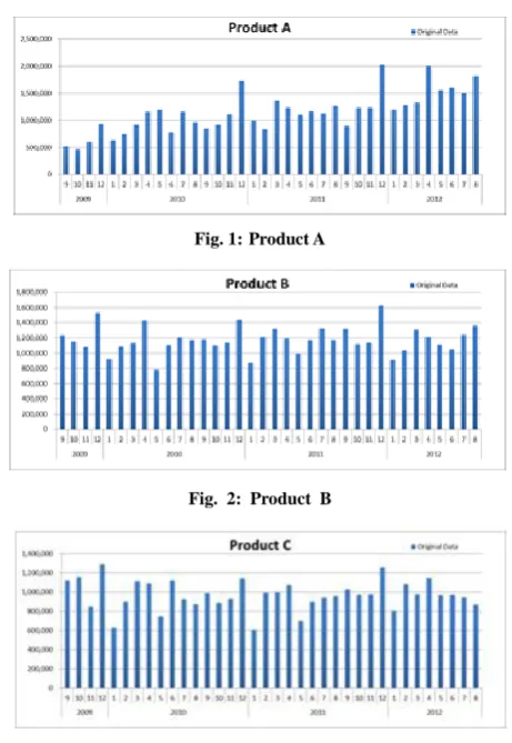
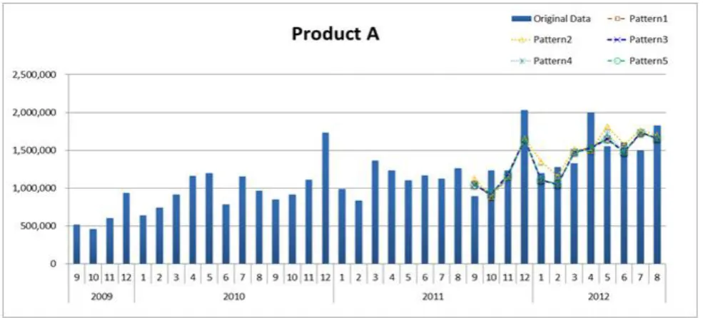
[image:3.595.314.545.389.724.2]

M a n u fa c t ur e r ’s d a t a o f s a ni t a r y ma t e r i a l s from September 2009 to August 2012 are analyzed. First of all, graphical charts of these time series data are exhibi ted in Fig. 1, 2,3.

Fig. 1:Product A

Fig. 2: Product B

Fig. 3: Product C

1 1

x

b

a

(4)

International Journal of Emerging Technology and Advanced Engineering

609 Analysis procedure is as follows. There are 36 monthly data for each case. We use 24 data(1 to 24) and remove trend by the method stated in 3. Then we calculate monthly ratio by the method stated in 4. After removing monthly trend, the method stated in 2 is applied and Exponential Smoothing Constant with minimum variance of forecasting error is estimated. Then 1 step forecast is executed. Thus, data is shifted to 2nd to 25th and the forecast for 26th data is executed consecutively, which finally reaches forecast of 36th data. To examine the accuracy of forecasting, variance of forecasting error is calculated for the data of 25th to 36th data. Final forecasting data is obtained by multiplying monthly ratio and trend. Forecasting error is expressed as:

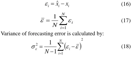
i i i



x

ˆ



x



(16)





N

i i

N

₁

1 _



(17)

Variance of forecasting error is calculated by:





2

1 2

1

1 _







N

i i

N





_ (18)

5.2 Trend Removing

Trend is removed by dividing original data by (12),(13),(14). The patterns of trend removal are exhibited in Table 1.

Table 1

The patterns of trend removal

Patter

n1



1,



2are set 0.5 in the equation (12) Patter

n2



1,



2are set 0.5 in the equation (13) Patter

n3



1is shifted by 0.01 increment in (12) Patter

n4



1is shifted by 0.01 increment in (13) Patter

n5

1

γ

and

γ

₂ are shifted by 0.01 increment in (1 4)

In pattern1 and 2, the weight of



₁,



₂,



₁,



₂ are set 0.5 in the equation (12),(13). In pattern3, the weight of



₁ is shifted by 0.01 increment in (12) which satisfy the range0



11.00. In pattern4, the weight

of



₁is shifted in the same way which satisfy the range0



11.00. In pattern5, the weight of



1and

2



are shifted by 0.01 increment in (14) which satisfy the range0



11.00,0



21.00.

The best solution is selected which minimizes the variance of forecasting error. Estimation results of coefficient of (9), (10) and (11) are exhibited in Table 2. Estimation results of weights of (12), (13) and (14) are exhibited in Table 3.

Table 2

Coefficient of (9),(10) and (11)

1st 2nd 3rd

1

a

b

₁

a

₂

b

₂

c

₂

a

3

b

3

c

3

d

3

Prod uct

A

27788.7 3087

644107.48 91

-1764.808 764

71908.94 997

452919.87 3

100.60240 4

-5537.398

914 110409.49

364641.26 35

Prod uct

B

900.569 5652

1154539.5 47

525.1695 5

-12228.66 919

1211432.9 15

-46.66049 195

2274.9379 98

-30085.63 945

1252377.4 97

Prod uct

C

-5731.7 87391

1027967.8 84

542.9100 258

-19304.53 804

1086783.1 37

-50.38907 413

2432.5003 06

-38588.43 671

[image:4.595.311.552.155.292.2] [image:4.595.47.278.313.419.2]

(5)

International Journal of Emerging Technology and Advanced Engineering

610

Table 3

Weights of (12), (13) and (14)

Monthly

ratio

Pattern1 Pattern2 Pattern3 Pattern4 Pattern5

1



2



1



2



1



2



1



2



1



2



3

Product A

Used 0.50 0.50 0.50 0.50 0.78 0.22 1.00 0.00 0.78 0.22 0.00

Not used 0.50 0.50 0.50 0.50 0.78 0.22 1.00 0.00 0.78 0.22 0.00

Product B

Used 0.50 0.50 0.50 0.50 0.57 0.43 1.00 0.00 0.57 0.43 0.00

Not used 0.50 0.50 0.50 0.50 0.57 0.43 1.00 0.00 0.57 0.43 0.00

Product C

Used 0.50 0.50 0.50 0.50 0.27 0.73 0.18 0.82 0.18 0.00 0.82

Not used 0.50 0.50 0.50 0.50 0.27 0.73 0.18 0.82 0.18 0.00 0.82

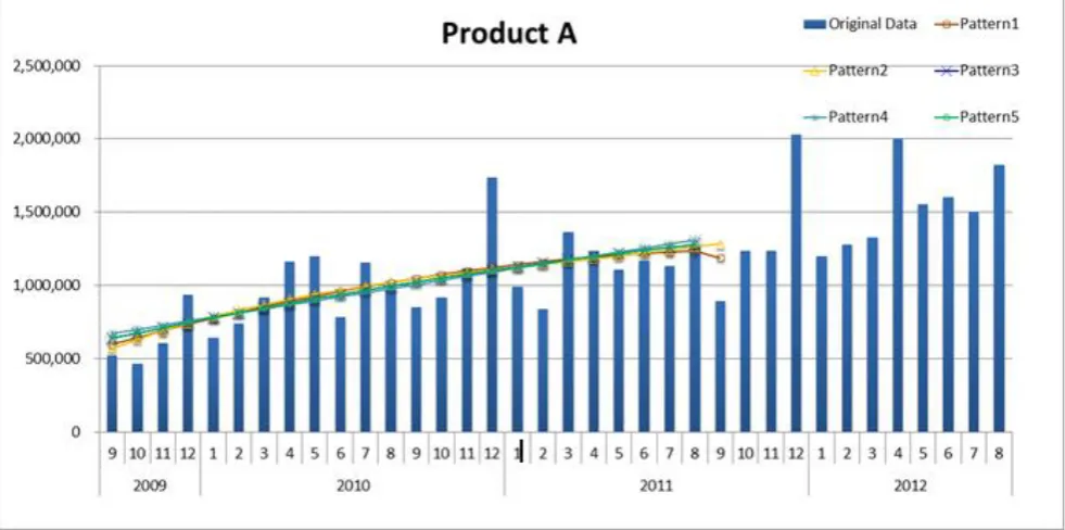
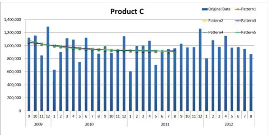
[image:5.595.49.574.169.317.2]

Graphical chart of trend is exhibited in Fig. 4, 5, 6 for the cases that monthly ratio is used.

[image:5.595.59.550.351.595.2]

(6)

International Journal of Emerging Technology and Advanced Engineering

[image:6.595.69.537.154.386.2]

611

Fig. 5: Trend of Product B

[image:6.595.71.539.429.664.2]

(7)

International Journal of Emerging Technology and Advanced Engineering

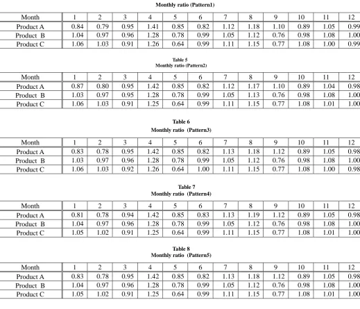
612 5.3 Removing trend of monthly ratio

After removing trend, monthly ratio is calculated by the method stated in 4. Calculation result for 1st to 24th data is exhibited in Table 4 through 8.

Table 4 Monthly ratio (Pattern1)

Month 1 2 3 4 5 6 7 8 9 10 11 12

Product A 0.84 0.79 0.95 1.41 0.85 0.82 1.12 1.18 1.10 0.89 1.05 0.99 Product B 1.04 0.97 0.96 1.28 0.78 0.99 1.05 1.12 0.76 0.98 1.08 1.00 Product C 1.06 1.03 0.91 1.26 0.64 0.99 1.11 1.15 0.77 1.08 1.00 0.99

Month 1 2 3 4 5 6 7 8 9 10 11 12

5.4 Estimation of Smoothing Constant with Minimum Variance of Forecasting Error

After removing monthly trend, Smoothing Constant with minimum variance of forecasting error is estimated utilizing (7).

[image:7.595.36.556.199.644.2]

(8)

International Journal of Emerging Technology and Advanced Engineering

613

Table 9

Estimated Smoothing Constant with Minimum Variance

Monthly ratio

Pattern1 Pattern2

1







₁



Product A Used

-0.0644

0.9353

-0.1109

0.8877

Not used

-0.0163

0.9837

-0.0403

0.9596

Product B Used

-0.0668

0.9329

-0.0721

0.9275

Not used

-0.3098

0.6529

-0.3182

0.6407

Product C Used

-0.0222

0.9777

-0.0002

0.9998

Not used

-0.2335

0.7521

-0.3066

0.6574

Monthly ratio

Pattern3 Pattern4 Pattern5

1







₁





₁



Product A Used

-0.0421 0.9578 -0.1243

0.8738 -0.0421 0.9578

Not used

-0.1050 0.8938 -0.0036

0.9964

-0.0495 0.9503

Product B Used

-0.0469 0.9530 -0.0033

0.9967 -0.0469 0.9530

Not used

-0.2971 0.6706 -0.3349

0.6156 -0.2971 0.6706

Product C Used

-0.0495 0.9504 -0.0076

0.9924 -0.0248 0.9752

Not used

-0.2451 0.7381 -0.2832

0.6896 -0.2451 0.7381

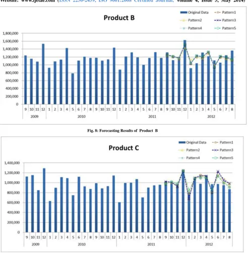
5.5 Forecasting and Variance of Forecasting Error Utilizing smoothing constant estimated in the previous section, forecasting is executed for the data of 25th to 36th data. Final forecasting data is obtained by multiplying monthly ratio and trend.

[image:8.595.38.553.165.402.2]

Variance of forecasting error is calculated by (18). Forecasting results are exhibited in Fig. 7, 8, 9 for the cases that monthly ratio is used.

[image:8.595.52.545.476.699.2]

(9)

International Journal of Emerging Technology and Advanced Engineering

[image:9.595.54.547.131.635.2]

614

Fig. 8: Forecasting Results of Product B

(10)

International Journal of Emerging Technology and Advanced Engineering

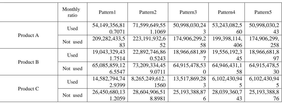
615 Variance of forecasting error is exhibited in Table 10.

Table 10 Variance of Forecasting Error

Monthly

ratio Pattern1 Pattern2 Pattern3 Pattern4 Pattern5

Product A

Used

54,149,356,81

0.7071

71,599,649,55

1.1069

50,998,030,24

3 53,243,082,5

60 50,998,030,2

43

Not used

209,282,433,5

83 223,191,932,6

52 174,906,299,2

58 199,398,114,

406 174,906,299,

258

Product B

Used

19,043,329,43

1.7514

22,892,746,86

0.5243

18,966,681,89

7 19,556,192,3

45 18,966,681,8

97

Not used

65,085,859,12

6.5547

73,209,334,45

9.0711

64,915,478,53

0 64,946,431,1

58 64,915,478,5

30

Product C

Used

14,582,794,74

2.9399

8,265,249,612.

1560

13,517,869,28

3 6,102,430,94

5 6,102,430,94

5

Not used

26,450,680,13

1.2059

28,604,906,51

8.8981

25,193,388,87

6 28,039,360,7

43 25,193,388,8

76

5.6 Remarks

In all cases, that monthly ratio was used had a better forecasting accuracy. Product A and Product B had a good result in 1st+2nd order with the case that monthly ratio was used, while Product C had a good result in 1st+3rd order with the case that monthly was not used. We can observe that monthly trend is relatively apparent in these cases.

VI. CONCLUSION

Correct sales forecasting is inevitable in industries. Focusing on the idea that the equation of exponential smoothing method(ESM) was equivalent to (1,1) order ARMA model equation, a new method of estimation of smoothing constant in exponential smoothing method was proposed before by us which satisfied minimum variance of forecasting error. Generally, smoothing constant was selected arbitrarily. But in this paper, we utilized above stated theoretical solution. Firstly, we made estimation of ARMA model parameter and then estimated smoothing constants. Thus theoretical solution was derived in a simple way and it might be utilized in various fields.

Furthermore, combining the trend removal method with this method, we aimed to improve forecasting accuracy. A mere application of ESM does not make good forecasting accuracy for the time series which has non-linear trend and/or trend by month. A new method to cope with this issue is required.

Therefore, utilizing above stated method, a revised forecasting method is proposed in this paper to improve forecasting accuracy. An approach to this method was executed in the following method. Trend removal by a linear function was applied to the manufacturer’s data of sanitary materials. The combination of linear and non-linear function was also introduced in trend removing. For the comparison, monthly trend was removed after that. Theoretical solution of smoothing constant of ESM was calculated for both of the monthly trend removing data and the non-monthly trend removing data. Then forecasting was executed on these data. In all cases, that monthly ratio was used had a better forecasting accuracy. Product A and Product B had a good result in 1st+2nd order with the case that monthly ratio was used, while Product C had a good result in 1st+3rd order with the case that monthly was not used. We can observe that monthly trend is relatively apparent in these cases.

Various cases should be examined hereafter. In the end, we appreciate Mr. Norio Funato for his helpful support of our study.

APPENDIX:

Estimation of smoothing constant in Exponential Sm oothing Method [12]

Comparing with (3) and (4), we obtain











1

[image:10.595.27.571.173.372.2]

(11)

International Journal of Emerging Technology and Advanced Engineering

616 From (1), (6),

Therefore, we get

From above, we can get estimation of smoothing constan t after we identify the parameter of MA part of ARMA mod el. But, generally MA part of ARMA model become non-lin earequations which are described below. Let (4) be

i t p i i t

t

x

a

x

_ 







1

~

_(A-2)

j t q j j t

t

e

b

e

x

_ 







1

~

(A-3)

We express the autocorrelation function of

x

~

_t as r~ k

and from (A-2), (A-3), we get the following non-linear equations which are well known[3].



   











q j j e j k k q j j e k

b

r

q

k

q

k

b

r

0 2 2 0 0 2

~

)

1 (

0 )

(

~



(A-4)

For these equations, recursive algorithm has been developed. In this paper, parameter to be estimated is only

b1, so it can be solved in the following way. From (3) (4) (A-1) (A-4), we get





2 1 1 2 2 1 0 1 1

~

1 ~

1

e e

b

r

b

r

b

a

q

























(A-5)

If we set

0

~

r

_k k





(A-6)

the following equation is derived.

2 1 1 1

1 b

b







(A-7)

We can get b1 as follows.

1 2 1 1

2

4

1

1 









b

(A-8)

In order to have real roots,



₁must satisfy

2

1





(A-9)

From invertibility condition,

b

₁ must satisfy

1



b

From (A-7), using the next relation,







1 

0

1

2 1 2 1









b

(A-9) always holds. As

1





b



1

b

is within the range of

0

1 

₁





b

Finally we get

1 2 1 1 1 2 1 1

2

4

1

2

1

2

4

1

1 

















b

(A-10)

Which satisfy above condition.

REFERENCES

[1] Box Jenkins. (1994) Time Series Analysis Third Edition，Prentice Hall.

[2] R.G. Brown. (1963) Smoothing, Forecasting and Predict on of Discrete –Time Series, Prentice Hall.

[3] Hidekatsu Tokumaru et al. (1982) Analysis and Measurement –Theory and Application of Random data Handling, Baifukan Publishing.

[4] Kengo Kobayashi. (1992) Sales Forecasting for Budgeting, Chuokeizai-Sha Publishing.







1 

(12)

International Journal of Emerging Technology and Advanced Engineering

617

[5] Peter R.Winters. (1984) Forecasting Sales by Exponentially Weighted Moving Averages, Management Science，Vol6，No.3, pp. 324-343.

[6] Katsuro Maeda. (1984) Smoothing Constant of Exponential Smoothing Method, Seikei University Report Faculty of Engineering, No.38, pp. 2477-2484.

[7] M.West and P.J.Harrison. (1989) Baysian Forecastingand Dynamic Models，Springer-Verlag，New York.

[8] Steinar Ekern. (1982) Adaptive Exponential SmoothingRevisited， Journal of the Operational Research Society, Vol．32 pp．775-782. [9] F.R.Johnston. (1993) Exponentially Weighted Moving Average (EWMA) with Irregular Updating Periods, Journal of the Operational Research Society，Vol.44，No.7 pp．711-716.

[10] Spyros Makridakis and Robeat L.Winkler. (1983) Averages of Forecasts；Some Empirical Results，Management Science，Vol.29, No.9, pp. 987-996.

[11] Naohiro Ishii et al. (1991) Bilateral Exponential Smoothing of Time Series, Int.J.System Sci., Vol.12, No.8, pp. 997-988.

[12] Kazuhiro Takeyasu and Keiko Nagata.(2010) Estimation of Smoothing Constant of Minimum Variance with Optimal Parameters of Weight, International Journal of Computational Science Vol.4,No.5, pp. 411-425.

[13] Kazuhiro Takeyasu, Keiko Nagata, Yuki Higuchi. (2009) Estimation of Smoothing Constant of Minimum Variance And Its Application to Shipping Data With Trend Removal Method, Industrial Engineering ＆ Management Systems (IEMS),Vol.8,No.4, pp.257-263,

[14] Kazuhiro Takeyasu, Keiko Nagata, Yui Nishisako. (2010) A Hybrid Method to Improve Forecasting Accuracy Utilizing Genetic Algorithm And Its Application to Industrial Data, NCSP'10, Honolulu,Hawaii,USA

[15] Kazuhiro Takeyasu, Keiko Nagata, Kana Takagi. (2010) Estimation of Smoothing Constant of Minimum Variance with Optimal Parameters of Weight, NCSP'10, Honolulu,Hawaii,USA

[16] Kazuhiro Takeyasu, Keiko Nagata, Tomoka Kuwahara. (2010) Estimation of Smoothing Constant of Minimum Variance Searching Optimal Parameters of Weight, NCSP'10, Honolulu,Hawaii,USA [17] Kazuhiro Takeyasu, Keiko Nagata, Mai Ito, Yuki Higuchi (2010). A

Hybrid Method to Improve Forecasting Accuracy Utilizing Genetic Algorithm, The 11th APEIMS, Melaka, Malaysia

[18] Kazuhiro Takeyasu, Keiko Nagata, Kaori Matsumura. (2011) Estimation of Smoothing Constant of Minimum Variance and Its Application to Sales Data, JAIMS, Honolulu, Hawaii, USA [19] Hiromasa Takeyasu, Yuki Higuchi, Kazuhiro Takeyasu. (2012) A