An Accurate Power System Fault Classification and Location Algorithm for Series Compensated Line

(1)

International Journal of Emerging Technology and Advanced Engineering

Website: www.ijetae.com (ISSN 2250-2459,ISO 9001:2008 Certified Journal, Volume 6, Issue 3, March 2016)

107

An Accurate Power System Fault Classification and Location

Algorithm for Series Compensated Line

Deba Prasad Patra

Asst. Professor, Dept. Of EE, SSTC-SSGI, Bhilai-490020, C.G, India

Abstract—This paper studies the problem of fault location

and classification in a power system by fast identifying and locating the possible faults The proposed method uses the samples of half cycle duration of three phase currents (IR, IY

and IB) as features of support vector machine (SVM) to

accomplish the fault classification task. The feasibility of the proposed algorithm has been tested on a 300 km, 400kV series compensated transmission line through detailed digital studies using MATLAB for various test cases comprising of all the types of faults. The results indicate that the proposed technique is fast, accurate and robust for a wide variation in system and fault conditions.

Keywords— fault location, SVM, series Compensated Line

I. INTRODUCTION

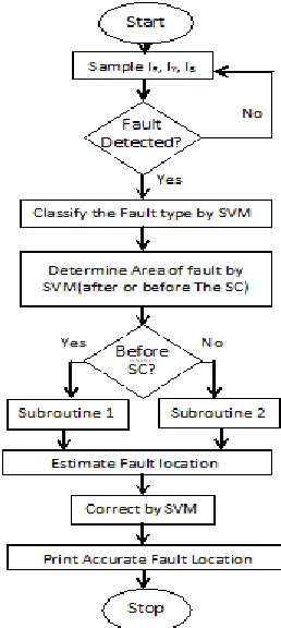
Overhead transmission lines are exposed to majority of short circuit faults causing a great economical loss to power system. Numerical protection enables one to implement elaborate fault classification and locating algorithm to digital distance relay or digital fault recorders or in stand-alone dedicated fault locating systems. Early and accurate measurement of fault have tremendous cost benefit. Many researchers have developed various fault classification and location algorithm [1-5]. The fault location algorithm is developed here as a ‗Two end fundamental frequency based technique‘ which uses the classified output of previous algorithm and takes into account both the series compensation effect and the reactance effect resulting from the remote end in feed. Series Capacitors (SC) and Metal Oxide Varistors (MOV) schemes are made equivalent for the fundamental frequency [7] . The method uses phase coordinates instead of symmetrical components. The steps of the algorithm are depicted in the flow diagram. The result of this algorithm is validated with the published works of Saha et al[1] and Dabbagh[2] which proves the accuracy of the developed technique here[3].

II. FAULT CLASSIFICATION TECHNIQUE

Let us consider a series compensated line as shown in figure 1 (a) [7] below with the following assumptions. The SCs and MOVs are installed at a distance x from the substation

Fig. 1 (a) Single line diagram of the system studied

Fig. 1 (b) Flow chart for estimating accurate fault location. 1.The shunt capacitances of the line are neglected at this

stage

[image:1.612.370.499.341.629.2]

(2)

International Journal of Emerging Technology and Advanced Engineering

108 3. The recorded voltage and current data cover the time

window when MOVs actually operate i.e., they are not short circuited by firing the air gaps.

4. The fault resistance, system impedance and equivalent electromotive forces are all constant during the fault. Accurate prediction of phases involved in the fault is essential for computing the fault distance as well as for proper isolation of faulty phase(s). For series compensated lines, the fault classification task becomes more complicated [3,4]. In the literature, various attempts have been made to solve this complex classification problem for series compensated lines using neural network, adaptive Kalman filtering, wavelet transform, and fuzzy logic based approaches[3].

2.1 Use of SVM in fault classification

In recent years, SVM has emerged as a very powerful tool to solve the classification and regression problems. For classification problems the SVMs try to find out an ‗optimal hyper-plane‘ to separate points according to their classes such that the separation between the classes is classed as maximum. Classification can be thought as predictions with only binary outcomes. The details of SVM can be followed from the existing literature [5].

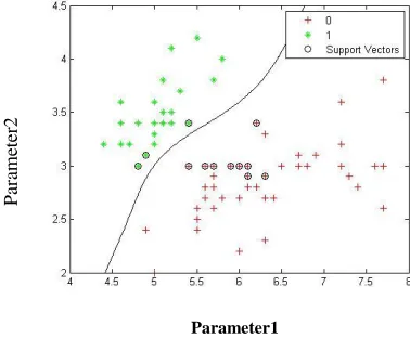
[image:2.612.332.521.142.298.2]

Once the training samples are obtained, the next step is to determine the most suitable Kernel function [4] (along with its associated parameters) and the optimal value of the regularization parameter for each SVM. In this work, these parameters have been set for each SVM separately. For this purpose each SVM, under study have been trained and tested with different types of Kernel functions, namely radial basis function (RBF), polynomial kernel function, linear kernel function etc and was found RBF kernel function being the best among all. Fig. 2 depicts the use of polynomial kernel function for classification of two different type data. The combination for which the maximum accuracy is obtained for that particular SVM is finally chosen.

Fig. 2 Classification of two types of data

Now the current waveform is sampled in a sampling frequency . As the sampling frequency is it would have 0.02 samples per cycle and 0.01 samples per half cycle. In the first stage the sampled half cycle is compared with the corresponding half cycle of non faulted wave form. The non faulted wave form and faulted wave forms are compared on the basis of three phase current parameters(Ia, Ib, Ic) . SVM classifies between non faulted and faulted wave form.

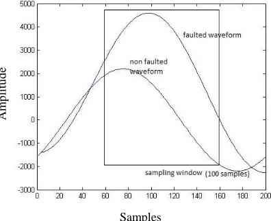
After the fault detection we go for classification. The faulted sample window is compared with all 10 SVMs and the appropriate fault is classified. In Figure 3 a faulted and non faulted wave form have been shown. The half cycle having the best classifiable range of value is taken into consideration. As we can see in the figure the best classifiable sample values lies in the range 60 to 160. Taking sampling frequency = 10kHz we can infer that a full cycle will have 200 samples and we take only a half cycle samples that is 100 no. of samples to classify between a faulted and non faulted wave.

P

ara

m

eter2

(3)

International Journal of Emerging Technology and Advanced Engineering

[image:3.612.326.550.112.246.2]

109 Fig. 3 Faulted and non-faulted waveform

III. FAULT LOCATING ALGORITHM

The algorithm as mentioned is developed in phase coordinates to handle the SCs and MOVs in convenient way i.e. the parameters of the equivalent branch depend upon the phase currents. In addition to this, it also enables us to locate faults in un-transposed series compensated lines [1].

3.1 Transmission line and Supplying systems

The local supplying system ‘A’ is represented by the matrix form in its electromotive forces and currents as follows:

(1)

For a completely transposed system the source impedance matrix becomes:

ZA (2)

ZAs = Self Impedance, ZAm = Mutual impedance which

are obtained from zero sequence (Z A0) and positive

sequence data (Z A1)using the relations below.

(3)

The same applies to the remote system ‘B’ (EB , ZB and

IB) and the line[3].

3.2 SCs and MOVs

The parallel connection of a SC and MOV is represented by the equivalent resistance Rv, and the reactance XV,

connected in series (as shown in Fig.4) [7].

For faults in front of SCs & MOVs (F1) (Fig.1) fault loops do not contain SCs and MOVs [7]. Therefore, it is analogous to the case of traditional uncompensated lines; the fault loop is of the form of resistive-inductive circuit (neglecting line shunt capacitances). SCs and MOVs even being placed outside fault loops; influence the fault loop impedance measurement to some extends by means of the remote line end infeed. It is worth noticing that the infeed has to be taken into account for fault location aimed at pin-pointing the fault position for post-fault inspection and repairs of the line. Generally the faults in front of SCs and MOVs (F1) are considered as not differing much from the faults on uncompensated lines.

For faults behind SCs & MOVs (F2) (Fig.1) the substantial difference appears for faults behind SCs & MOVs (F2) [1]. In this case the type of a fault, whether it is a phase-to-ground or a phase-to-phase fault, is important for considering the composition of a fault loop. For the phase-to-ground fault the fault loop contains the faulty segment of the line, one SC together with its MOV and the fault resistance. In the case of phase-to-phase faults, the fault loop impedance is being determined on the base of the fault current and the difference of phase voltages taken from the phases involved in a fault. Therefore, for phase-to-phase faults the fault loop contains two complexes of SCs and MOVs.

Involvement of SC and MOV or even two such complexes in the fault loop makes the fault loop a strongly nonlinear circuit. Equivalenting the SCs and MOVs for the fundamental frequency allows measuring the resistive inductive impedance of the fault loop which corresponds to the strict distance to a fault (if the infeed effect is neglected).

3.2.1 Fundamental Frequency Equivalenting

The voltage-current characteristic for the MOV [7] (Fig.4) is approximated as follows:

(4)

Am

p

li

tu

d

e

Samples

Fig. 4(a) SC and MOV in Parallel

[image:3.612.63.261.143.304.2]

(4)

International Journal of Emerging Technology and Advanced Engineering

110 P - Reference current VREF- Reference voltage

q – Exponent

Fig.5 V-I characteristics of MOV [7]

It is obvious that the values of resistance and the reactance depend on the amplitude of current flowing through the device. Basically the equivalence is done in analytical and simulation method [3], where the former is opted in this paper [6].

With functions RV(IV), XV(IV) known, the SCs and their

MOVs are described in a method by the current dependent impedance matrix:

(5)

(6)

Where, IV is a vector of currents flowing through the

bank.

3.3 Rough Estimation of fault location

For Faults before SC (F1): The distance to fault can be calculated as below

(7)

For Faults after SC (F2): The distance to fault can be calculated as below

(8)

3.4 Selection of Algorithm

As seen, fault may be located in front of SC or after the SC. The formulation for the two types of fault being different, the correct subroutine has to be chosen for correct fault distance determination. This is accomplished by SVM. The feature used for classification of fault area is sending end and receiving end current.

This implies there is no need of calculation of fault resistance for selecting correct fault area which is an improvement to the existing literature [1].

3.5 Correction of Estimated Fault location

The estimated fault location is made accurate by using SVM. For fault at each kilometer one data set is generated hence 300 datasets are generated. This dataset is generated using MATLAB software. Now the SVM is trained with this data set and tested for various cases. More over the accuracy of distance to fault can be increased with decreasing the fault step (e.g. at each 100 m a fault can be simulated to generate more no of data sets hence more accuracy.).

IV. SUMMARY OF DATA AND MEASUREMENTS The algorithm needs the following data and measurements:-

 Line impedance (3x3 phase matrix)

 Local source impedance (3x3 phase matrix)

 Remote source impedance (3x3 phase matrix)

 Location of compensating bank (p)

 Equivalenting branch for the SCs and MOVs (two functions or tables);

 Type of fault

 Three phase local voltage (phasors)

 Three phase local currents including their pre-fault values( phasors )

V. CASE STUDY

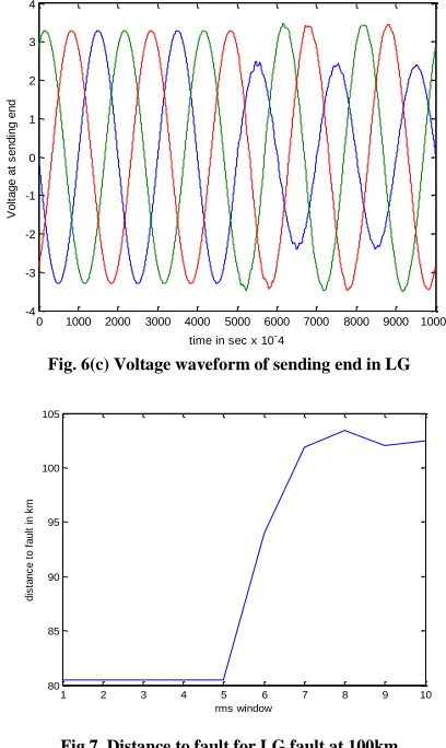
The algorithm described is implemented for a 300km, 400kV line with specifications given in Appendix-1. Fig. 6(a) depicts the MATLAB SIMULINK Model of the Transmission line. The system current and voltage waveform for L-G fault at sending end is shown in Fig. 6(b-c). Fig.7 shows the result of distance to L-G fault at a position 100 km from the sending end and Table.1 shows the rough estimation and corrected distance to fault for various fault condition The simulation has been done in minimum possible time [1-2].

(5)

International Journal of Emerging Technology and Advanced Engineering

111

0 1000 2000 3000 4000 5000 6000 7000 8000 9000 10000 -4 -3 -2 -1 0 1 2 3 4x 10

5

time in sec x 10-₄

V o lt a g e a t s e n d in g e n d

1 2 3 4 5 6 7 8 9 10

80 85 90 95 100 105 rms window d is ta n c e t o f a u lt i n k m

In the SVM classifier for each sampling window 50% data are used for training the data sets and the rest are tested which provide the accuracy with which wave forms are classified. The type of fault determined by SVM classifier is fed to the ‗Fault Locating Algorithm‘. Now the area of fault is first determined again using SVM. Fault locating algorithm along with different data such as (faulted voltage/current, pre fault voltage/current) proceeds to the estimation of fault. Now the exact location is determined using the SVM e.g. if the rough estimation says there is fault at 100.5 km then the exact fault distance is calculated using training data sets( i.e. simulated for each km. ). The fault position having most similarity measure is depicted as the fault location.

Fig. 6(a) Transmission Line Model

Fig. 6(b) Current wave form of sending end in LG fault

[image:5.612.339.543.148.490.2]

Fig. 6(c) Voltage waveform of sending end in LG

Fig.7 Distance to fault for LG fault at 100km Table 1

Results of simulation for different faults

Fault type

Rf

(Ώ) Actual Fault Distanc e (km) positio n of SC (km) Estimate

d Fault

Distance (km) Corrected Fault distance (km)

a-g 1

10

100 150 101.75

105.84

100 100

b-g 1

10

100 150 99.14

103.11

100

c-g 1

10

100 150 96.79

102.18

100 100

a-g 1

10

200 150 200.77

195.56

200 200

b-g 1

10

200 150 198.5

194.18

200 200

c-g 1

10

200 150 196.21

191.66

[image:5.612.50.282.312.491.2]

(6)

International Journal of Emerging Technology and Advanced Engineering

112 VI. CONCLUSIONS

In this paper a new SVM based fault classification algorithm and an accurate algorithm for locating faults in series compensated lines has been presented. The proposed fault classification technique uses samples of phase currents as input features of SVMS for identification of faulty phases. The accuracy of the algorithm was tested on various data sets and was found very accurate. The proposed technique can be used as an attractive and effective approach for alternative classification algorithm for power system faults. When transmission and distribution system are going to be integrated the proposed approach will no doubt be a smart technique to add reliability in energy management system.

APPENDIX-I

REFERENCES

[1] M.M. Saha, J. Jzykowski, E. Rosolowski, and B. Kasztenny,1999, ―A new accurate fault locating algorithm for series compensated lines‖, IEEE Trans. Power Deliv. Vol.14 (3), pp. 789–795. [2] Majid Al-Dabbagh , and Sarath K. Kapuduwage, 2005, ―Using

instantaneous values for estimating fault locations on series compensated transmission lines‖, Electric Power Systems Research 76, pp. 25–32.

[3] Shibashis Sahu , 2011, ―An accurate fault classification and fault locating algorithm of a series compensated transmission line‖, U.G. Project thesis, VSSUT, Burla,

[4] Urmil B. Parikh ,Biswarup Das, and Rudraprakash Maheshwari, 2010, ―Fault classification technique for series compensated transmission line using support vector machine‖, Electrical Power and Energy Systems Vol. 32, pp. 629–636.

[5] Christopher J.C. Burges, 1998, “A Tutorial on Support Vector Machines for Pattern Recognition‖, Kluwer Academic Publishers, Boston.

[6] M.M. Saha ,J. Jzykowski, E. Rosolowski, and B. Kasztenny, Research Gate online 02/2001, ―Fundamental frequency Equivalenting of series capacitors with MOVs in a Series compensated line under Fault condition‖.

[7] M.M. Saha ,J. Jzykowski, E. Rosolowski, and B. Kasztenny, Research Gate online,1999, ―Differential equation based impedance measurement for series-compensated lines‖.

Source data at both sending and receiving ends

Positive sequence impedance

Zero sequence impedance

Frequency

1.31 + j15.0 X.

2.33 + j26.6 X.

50 Hz.

Transmission-line data

Length

Voltage

Positive-sequence impedance

Zero-sequence impedance