Quasilinearization for nonlinear boundary value problems for delay type difference equations with maxima

(1)

R E S E A R C H

Open Access

Quasilinearization for nonlinear boundary

value problems for delay-type difference

equations with maxima

Snezhana Hristova

*

_{and Angel Golev}

*_{Correspondence:}

[email protected] Plovdiv University, Tzar Asen 24, Plovdiv, 4000, Bulgaria

Abstract

The paper deals with an approximate method for solving a mixed boundary value problem for nonlinear diﬀerence equations containing a maximum of the unknown function over a past time interval. Every successive approximation to the unknown solution is the unique solution of an appropriately constructed initial value problem for a linear diﬀerence equation with maxima, and an algorithm for its explicit obtaining is suggested. Also, each approximation is a lower/upper solution of the given mixed problem. The rapid convergence of the successive approximations is proved. The suggested algorithm is realized as a computer program and it is applied to an example.

MSC: 39A23; 39A99; 65Q10

Keywords: delay-diﬀerence equations with maxima; boundary value problem; approximate solution; computer realization

1 Introduction

In the last few decades great attention has been paid to automatic control systems and their applications to computational mathematics and modeling. Many problems in the control theory correspond to the maximal deviation of the regulated quantity. Discrete modeling of such kind of problems is done adequately by difference equations with max-ima over a past time discrete interval. These difference equations are a part of the set of difference equations with delays. Meanwhile, the delays have recently been found crucial in many areas such as neuronal dynamics. For example, the effects of periodic subthresh-old pacemaker activity and time-delayed coupling on stochastic resonance over scale-free neuronal networks are studied in []; the effects of spatiotemporal additive noise on the spatial dynamics of excitable neuronal media that is locally modeled by a two-dimensional map are considered in []; the discrete model of the movement of eukaryotic cells regu-lated by a process of phase separation of two competing enzymes on the cell membrane is studied in []; front propagation and synchronization transitions in dependence on the information transmission delay and coupling strength over scale-free neuronal networks with different average degrees and scaling exponents are investigated in [].

The presence of the maximum function over a discrete past time interval in the dis-crete equation requires not only more complicated calculations but also a development of new methods for qualitative investigations of the behavior of their solutions as well as

(2)

approximate methods for their solving. The character of the maximum function leads to a variety of different types of difference equations. The properties of solutions of some special types of difference equations with maxima are studied in [–]. In several papers various types of boundary value problems for difference equations have been studied and the monotone iterative method has been applied. For example, in [, ] first-order differ-ence equations are studied; in [] some criteria for existdiffer-ence and uniqueness results for nth order anti-periodic difference equations are developed; in [] a generalized delay dif-ference equation is studied by lower and upper solutions, but the problem consists only of a boundary condition, which does not get uniqueness of the solution; the global boundary value problem for difference equations without any kind of delay is well studied in []; in [] a nonlinear boundary value problem for a delay difference equation with one delay is studied by the monotone iterative method; in [] an approximate method with a rapid convergence is applied to an initial value problem for difference equations with maxima. Also, in [], the monotone iterative technique is applied to a periodic boundary value problem for difference equations with maxima, but the successive approximation is solu-tions of periodic boundary value problems, which are practically difficult to be obtained. Approximate methods for various problems for differential equations with maxima are proved and applied in [–].

In the paper a nonlinear diﬀerence equation of delayed type is considered. The studied equation generalizes the well-known problems in several ways:

- at each current time the value of unknown function is included in both parts of the equation, so the equation could not be solved recursively;

- the delays are without any restrictions;

- the boundary condition is set up in a very general way and it involves many other cases, which are studied in the literature (see, for example, the above-mentioned papers).

The main purpose of the paper is to establish comparison results which allow us to use upper and lower solutions in order to build two convergent monotonic sequences of func-tions with discrete domains. Each term of these sequences is a solution of an appropriately constructed initial value problem for a linear diﬀerence equation with maxima. An algo-rithm for solving these initial value problems is given. Also, each term of both sequences is a lower/upper solution of the given nonlinear boundary value problem. The limits of both sequences coincide to the solution of a given problem and the rapid convergence of both sequences is proved. Also, the algorithm is computerized and it is applied to a particular example to show the advantages of the suggested approximate method.

2 Statement of the problem

LetR+= [,∞),Zbe the set of all integers. For anyc,b∈Z:c<b, we denoteZ[c,b] ={z∈

Z:c≤z≤b}.

Leta,T∈Z:T>a+ ,r,p∈Z[,T–a] andh∈Z:h>  be ﬁxed.

Consider the following mixed boundary value problem for a nonlinear delay-diﬀerence equation with ‘maxima’ (MBVP):

u(k– ) =f

k,u(k),uτ(k)

,uτ(k)

, . . . ,uτr(k)

, max s∈Z[k–h,k]u(s)

(3)

u(k) =ϕ(k) fork∈Z[a–h+ ,a– ], () u(a) =gu(T–λ),u(T–λ), . . . ,u(T–λp),u(T)

, ()

whereu∈R,u(k– ) =u(k) –u(k– ),f :Z[a+ ,T]×Rr+_→_R_,_g_:_Rp+_→_R_,_τ m(k) :

Z[a+ ,T]→Z[a+  –h,T]:k–h≤τm(k)≤k,m= , , . . . ,r,λj∈Z[,T–a],j= , , . . . ,p,

andϕ:Z[a–h+ ,a– ]→R.

Any solution of MBVP ()-() is a ﬁnite sequence ofT–a+hreal numbers, and we consider it as a real-valued function with a discrete domain.

The presence of delaysτm generalizes the type of the considered diﬀerence equation

since the function f could depend on diﬀerent delays at any pointk. In the caser=h andτj(k) =k–j,j= , . . . ,r, the right-hand side of () is reduced tof(k,u(k–h),u(k–h+

), . . . ,u(k– ),u(k),maxs∈Z[k–h,k]u(s)). For some other particular cases, see equation ()

of the paper.

The presence of both delays and the maximum function in the equation leads to a new statement of the problem, which involves both the boundary condition and the initial con-dition. Problem ()-() covers many diﬀerent problems for diﬀerence equations with delays and maxima such as the initial value problem, the periodic boundary value problem, the linear boundary value problem.

3 Preliminary notes, basic notations and deﬁnitions Notem_i₌_nai=  and

m

i=nai= , wherem<n<∞andaj∈R,j∈Z[m,n].

For any functionF∈C₍_I_,_R_),_I_⊂_Rr+_,_V_{= (}_v

,v, . . . ,vr+), we denote byFvj(V) the ﬁrst

derivative ofF(V) with respect to itsjth argument, and byFvjvk(V) the second derivative

ofF(V) with respect to itsjth andkth arguments. We introduce the following notations:

χu(T)=u(T–λ),u(T–λ), . . . ,u(T–λp),u(T)

,

Uuτ(k)=uτ(k)

,uτ(k)

, . . . ,uτr(k)

,

uτ(k)=u(k),Uuτ(k), max s∈Z[k–h,k]u(s)

, k∈Z[a+ ,T].

Using the above notations, the right-hand sides of equation () and boundary condition () could be written in a simpler way:f(k,(u(τ(k)))) andg(χ(u(T))).

We will use the normu=max{|u(k)|:k∈Z[a–h+ ,T]}.

Letα,β:Z[a+  –h,T]→Rbe given functions such thatα(k)≤β(k). We introduce the following sets:

S(α,β) =u:Z[a–h+ ,T]→R:α(k)≤u(k)≤β(k),k∈Z[a–h+ ,T] , W(α,β) =x∈Rp+:χα(T)≤x≤χβ(T) ,

k(α,β) =

V∈Rr+:ατ(k)≤V≤βτ(k) , k∈Z[a+ ,T].

(4)

Deﬁnition [] The functionα:Z[a–h+ ,T]→Ris called a lower (upper) solution of MBVP ()-() if

α(k– )≤(≥)fk,α(k),ατ(k)

,ατ(k)

, . . . ,ατr(k)

, max s∈Z[k–h,k]α(s)

fork∈Z[a+ ,T],

α(k)≤(≥)ϕ(k) fork∈Z[a–h+ ,a– ],

α(a)≤(≥)gα(T–λ),α(T–λ), . . . ,α(T–λp),α(T)

.

4 Linear delay difference inequalities with maxima

We will consider the following linear diﬀerence inequality with ‘maxima’:

u(k– )≤K+Q(k)u(k) +

r

j=

Cj(k)u

τj(k)

+q(k) max

s∈Z[k–h,k]u(s), k∈Z[a+ ,T],

u(k)≤K, k∈Z[a–h+ ,a],

()

whereKis a nonnegative constant.

The inequalities () are the base of the main proof, and we will obtain a solution of () in an explicit form.

Lemma  Let the following conditions be fulﬁlled:

. The delaysτj:Z[a+ ,T]→Z[a+  –h,T],j∈Z[,r]are such thatk–h≤τj(k)≤k, k∈Z[a+ ,T].

. The functionsq,Q,Cj:Z[a+ ,T]→R+,j∈Z[,r],and

˜

S(k)≡q(k) +Q(k) +

r

j=

Cj(k) <  fork∈Z[a+ ,T]. ()

. The functionu:Z[a+  –h,T]→R+satisﬁes inequalities().

Then for k∈Z[a+ ,T]the inequality u(k)≤Kθ(k)holds,where

θ(k) = _k 

j=a+ –S˜(j)

+

k

j=a+



k

ξ=j –S˜(ξ)

. ()

Proof From inequality () we obtain

u(k)≤

k

j=a+

K+Q(j)u(j) +

r

i=

Ci(j)u

τi(j)

+q(j) max s∈Z[j–h,j]u(s)

,

(5)

Deﬁne a functionz:Z[a+  –h,T]→R+by the equalities

z(k) =

⎧ ⎪ ⎪ ⎨ ⎪ ⎪ ⎩

k

j=a+{K+u(j– ) +Q(j)u(j)

+r_i_=Ci(k)u(τi(j)) +q(j)maxs∈Z[j–h,j]u(s)}, k∈Z[a+ ,T],

K, k∈Z[a+  –h,a].

The function z(k) is nondecreasing and u(k) ≤ z(k), u(τj(k)) ≤ z(τj(k)) ≤ z(k), maxs∈Z[k–h,k]u(s)≤maxs∈Z[k–h,k]z(s) =z(k) fork∈Z[a+ ,T],j= , , . . . ,r.

From the deﬁnition ofz(k) and the ﬁrst inequality in (), we obtain

 –q(k) –Q(k) –

r

j=

Cj(k)

z(k)≤K+z(k– ), k∈Z[a+ ,T]. ()

By mathematical induction from (), condition  and the deﬁnition ofz(k), we prove the

claim.

In the case when all delaysτj(k) <kfork∈Z[a+ ,T], condition  of Lemma  could be

changed by a simpler one.

Lemma  Let the following conditions be fulﬁlled:

. The delaysτj:k–h≤τj(k) <kfor allj∈Z[,r]andk∈Z[a+ ,T].

. The functionsq,Q,Cj:Z[a+ ,T]→R+,j= , , . . . ,r,and

S(k)≡q(k) +Q(k) <  fork∈Z[a+ ,T]. () . The functionu:Z[a+  –h,T]→R+satisﬁes inequalities().

Then for k∈Z[a+ ,T]the inequality u(k)≤Kξ˜(k)holds,where

˜

ξ(k) =

k

s=a+

 +r_j_=Cj(s)

 –S(s) +

k

s=a+

_k

ξ=s+

 +r_j_=Cj(ξ)

 –S(ξ)



 –S(s). ()

Corollary  Let conditionsandof Lemma/Lemmabe fulﬁlled,and let the function u:Z[a+  –h,T]→R+satisfy inequalities()for K= .

Then u(k)≤for all k∈Z[a–h+ ,T].

5 Linear delay difference equations with maxima

In connection with the computer realization of the suggested method, we will give an al-gorithm for exact solution of the initial value problem for the scalar linear delay-diﬀerence equation with ‘maxima’:

u(k– ) =Q(k)u(k) +q(k) max s∈Z[k–h,k]u(s)

+

r

j=

Cj(k)u

τj(k)

+P(k), k∈Z[a+ ,T], ()

(6)

whereQ,P:Z[a+,T]→R,q,Cj:Z[a+,T]→R+forj= , , . . . ,r,ψ:Z[a+–h,a]→R

andτm(k) :Z[a+ ,T]→Z[a+  –h,T]:k–h≤τm(k)≤kform= , , . . . ,r.

We will consider two cases with respect to the type of delaysτj.

Case : Let the inequalityτj(k) <khold for allj∈Z[,r],k∈Z[a+ ,T]. Additionally, we

assume that inequality () is satisﬁed for allk∈Z[a+ ,T].

Assume that the valuesu(k) of the unknown solution are obtained for allk∈Z[a–h+ ,m], wherem<T. Now letk=m+ .

Case .: Let the following inequality be satisﬁed:

P(k) +r_j_=Cj(k)u(τj(k)) +u(k– )

 –Q(k) –q(k) ≥max

u(k–l) :l= , , . . . ,h . ()

Thus,max_s_∈_Z_[_k_–_h_,_k_]u(s) =u(k). Then the unique solution of IVP (), () is

u(k) =P(k) +

r

j=Cj(k)u(τj(k)) +u(k– )

 –Q(k) –q(k) . ()

Case .: Let inequality () be not satisﬁed for alll∈Z[,h]. Therefore, there exists m∈Z[,h] such thatmax_s_∈_Z_[_k_–_h_,_k_]u(s) =u(k–m). ThenQ(k)≤Q(k) +q(k) <  and the unique solution of IVP (), () is

u(k) =P(k) +

r

j=Cj(k)u(τj(k)) +u(k– ) +q(k)u(k–m)

 –Q(k) . ()

Case : Let there exist at least one j∈Z[,r] andk∈Z[a+ ,T] such that τj(k) =k.

Additionally, we assume that inequality () is satisﬁed for allk∈Z[a+ ,T].

Assume that the valuesu(k) of the unknown solution are obtained for allk∈Z[a–h+ ,m], wherem<T. Now letk=m+ .

Let there exist integersjs∈Z[,r] :τjs(k) =kfors∈Z[,m] andτj(k) <kforj=js,s∈

Z[,m]. Equation () is reduced to

 –Q(k) –

m

s=

Cjs(k)

u(k)

=u(k– ) +

r

i=,i=js,s∈Z[,m]

Ci(k)u

τi(k)

+q(k) max

s∈Z[k–h,k]u(s) +P(k). ()

Case .: Let the following inequality be satisﬁed:

P(k) +r_i_=,_i₌_j_s_,_s_∈_Z_[,_m_]Ci(k)u(τi(k)) +u(k– )

 –Q(k) –m_s_=Cjs(k) –q(k)

≥u(k–s), s∈Z[,h]. ()

Therefore,maxs∈Z[k–h,k]u(s) =u(k), and from () we obtain the solution

u(k) =P(k) +

r

i=,i=js,s∈Z[,m]Ci(k)u(τi(k)) +u(k– )

 –Q(k) –m_s_=Cjs(k) –q(k)

. ()

(7)

Therefore, there existsm∈Z[,h] such thatmaxs∈Z[k–h,k]u(s) =u(k–m).

Then the unique solution of problem (), () is given by

u(k) =P(k) +

r

i=,i=js,s∈Z[,m]Ci(k)u(τi(k)) +u(k– ) +q(k)u(k–m)

 –Q(k) –m_s_=Cjs(k)

. ()

6 Method of quasilinearization

We will apply the method of quasilinearization to obtain the approximate solution of MBVP ()-().

Theorem  Let the following conditions be fulﬁlled:

. The delaysτj(k) :k–h≤τj(k)≤kfor allj∈Z[,r]andk∈Z[a+ ,T].

. The functionf:Z[a+ ,T]×Rr+_→_R_{and for any}_k_∈_Z_[_a_{+ ,}_T_]_and

V∈k(α,β),the equalityf(k,V) =F(k,V) –G(k,V)holds,where the functions

F(k,V),G(k,V)are twice continuously diﬀerentiable with respect to any component ofVand the following inequalities are valid fork∈Z[a+ ,T],V∈k(α,β):

Fvivj(k,V)≥, Gvivj(k,V)≥, fori,j∈Z[,r+ ], ()

Fvj

k,α(k)

≥Gvj

k,β(k)

, j= , , . . . ,r+ , ()

r+

j=

Fvj

k,β(k)

–Gvj

k,α(k)

< . ()

. The functiong∈C₍_W₍_α

,β),R)is nondecreasing with respect to all its arguments.

. The functionsα,β:Z[a+  –h,T]→R,αis a lower solution,βis an upper solution of MBVP()-(),andα(k)≤β(k)fork∈Z[a+  –h,T].

Then there exist two sequences of functions{αn}∞n=,{βn}∞n=such that

(a) αn:Z[a+  –h,T]→R(n= , , . . .)are lower solutions of MBVP()-().

(b) βn:Z[a+  –h,T]→R(n= , , . . .)are upper solutions of MBVP()-().

(c) α(k)≤α(k)≤ · · · ≤αn(k)≤ · · · ≤βn(k)≤ · · · ≤β(k)≤β(k).

(d) Both sequences are convergent onZ[a+  –h,T]and their limits

u(k) =lim_n_→∞αn(k)andv(k) =limn→∞βn(k)are solutions of MBVP()-()in S(α,β).In the case of uniqueness,both limits coincide with this solution.

(e) The convergence is semi-quadratic,i.e.,there existλi(k),μi(k),νi(k) > ,i= , ,such that

x(k) –αn(k)≤λ(k)x–αn+μ(k)x–αn+ν(k)x–βn, βn(k) –x(k)≤λ(k)x–βn+μ(k)x–αn+ν(k)x–βn.

Proof We will give an algorithm for construction of successive approximations to the exact unknown solution of MBVP ()-().

Assume that the functionsαj(k),βj(k) :Z[a+  –h,T]→R,j= , , . . . ,n, are constructed

so that the following conditions are satisﬁed:

(H) αj(k)≥αj–(k)andβj(k)≤βj–(k)fork∈Z[a+  –h,T];

(H) αj(k)≤βj(k)fork∈Z[a+  –h,T];

(8)

(H) functionsαj,βjare lower and upper solutions of MBVP ()-(), respectively.

Consider both initial value problems (IVP) for the linear diﬀerence equations with ‘max-ima’:

x(k– ) =Qn(k)x(k) + r

m=

C_m(n)(k)xτm(k)

+qn(k) max s∈Z[k–h,k]x(s)

+Pn

k,αn(k)

, k∈Z[a+ ,T], () x(k) =ϕ(k) –knLn, k∈Z[a+  –h,a– ],

x(a) =gχαn(T)

,

()

and

x(k– ) =Qn(k)x(k) + r

m=

C(n)

m (k)x

τm(k)

+qn(k) max s∈Z[k–h,k]x(s)

+Pn

k,βn(k)

, k∈Z[a+ ,T], () x(k) =ϕ(k) +pnMn, k∈Z[a+  –h,a– ],

x(a) =gχβn(T)

,

()

where

Ln= min s∈Z[a–h+,a–]

ϕ(s) –αn(s)

, Mn= min s∈Z[a–h+,a–]

βn(s) –ϕ(s)

,

kn=min

Ln,

 n

, pn=min

Mn,

 n

,

andPn,Qn,qn,Cm:Z[a+ ,T]→R,m= , , . . . ,r, are deﬁned by

Pn

k,u(k)=fk,u(k)–Qn(k)u(k) – r

m=

C_m(n)(k)uτm(k)

–qn(k) max s∈Z[k–h,k]u(s),

Qn(k) =Fv

k,αn(k)

–Gv

k,βn(k)

≥, qn(k) =Fvr+

k,αn(k)

–Gvr+

k,βn(k)

≥, C_m(n_–) (k) =Fvm

k,αn(k)

–Gvm

k,βn(k)

, m= , , . . . ,r+ .

From inequalities () andαn(k)≥α(k),βn(k)≤β(k),k∈Z[a+  –h,T], it follows that

qn(k)≥. From inequalities (), () we get that the functionsQn,qn,Cm(n–) satisfy () for

k∈Z[a+ ,T]. IVPs (), () and (), () have unique solutionsαn+(k) andβn+(k),

respectively, which are deﬁned on the intervalZ[a+  –h,T].

From condition (H), forj=n, the constantsLn,Mn,kn,pn≥ follow.

Deﬁne a functionp:Z[a+  –h,T]→Rbyp(k) =αn(k) –αn+(k).

Letk∈Z[a+  –h,a– ]. From () we getϕ(k) –αn(k)≥Lnand

(9)

Now, letk=a. Then from (H) forj=nwe get

p(a) =αn(a) –g

χαn(T)

≤. ()

Letk∈Z[a+ ,T]. From the choice of the functionαnand equation () for the function αn+, we get

p(k– )≤Qn(k)p(k) + r

j=

C(_jn)(k)p

τj(k)

+qn(k) max

s∈Z[k–h,k]p(s). ()

According to Corollary , from inequalities ()-() it follows thatp(k)≤ fork∈

Z[a+  –h,T],i.e.,αn(k)≤αn+(k) fork∈Z[a+  –h,T].

Similarly, we proveβn(k)≥βn+(k) fork∈Z[a+  –h,T],i.e., condition (H) is satisﬁed

forj=n+ .

Now, we will prove that the functionαn+is a lower solution of MBVP ()-().

Letk∈Z[a+  –h,a– ]. From () we getαn+(k) =ϕ(k) –knLn≤ϕ(k).

Letk=a. From the proved above and condition  of Theorem , the inequalityαn+(a) =

g(χ(αn(T)))≤g(χ(αn+(T))) holds.

Letk∈Z[a+ ,T]. Then we obtain

αn+(k– ) = (Fv

k,αn(k)

–Gv

k,βn(k)

αn+(k) –αn(k)

+

r

j=

C(_jn)(k)αn+

τj(k)

–αn

τj(k)

+Fvr+

k,αn(k)

–Gvr+

k,βn(k)

× max

s∈Z[k–h,k]αn+(s) –s∈Zmax[k–h,k]αn(s)

+fk,αn(k)

–fk,αn+(k)

≤fk,αn+(k)

.

Similarly, we prove thatβn+(k) is an upper solution of MBVP ()-().

Now, we will prove (H) forj=n+ . Deﬁne a functionp:Z[a+  –h,T]→Rby the

equalityp(k) =αn+(k) –βn+(k).

Letk∈Z[a+  –h,a– ]. Thenp(k) =ϕ(k) –knLn–ϕ(k) –pnMn≤.

Also, from condition  of Theorem  and (H) forj=n, we getp(a) =g(χ(αn(T))) – g(χ(βn(T)))≤.

Now, letk∈Z[a+ ,T]. Then for the functionp(k) we get

p(k– ) =f

k,αn(k)

–fk,βn(k)

–Qn(k)

βn+(k) –βn(k)

+

r

j=

C(_jn)(k)αn+

τj(k)

–αn

τj(k)

+Qn(k)

αn+(k) –αn(k)

–

r

j=

C_j(n)(k)βn+

τj(k)

–βn

(10)

+qn(k)

max

s∈Z[k–h,k]αn+(s) –s∈Zmax[k–h,k]αn(s)

–qn(k)

max

s∈Z[k–h,k]βn+(s) –s∈Zmax[k–h,k]βn(s)

≤Qn(k)p(k) + r

j=

C_j(n)(k)p

τj(k)

+qn(k) max

s∈Z[k–h,k]p(s). ()

According to Corollary , the inequality p(k)≤ holds fork∈Z[a+  –h,T],i.e., αn+(k)≤βn+(k) fork∈Z[a+  –h,T].

Therefore,αn+,βn+∈S(α,β).

For any ﬁxedk∈Z[a+  –h,T], the sequences{αn}∞n=and{βn}∞n=are monotone

non-decreasing and monotone nonincreasing, respectively, and they are bounded by the func-tionsαandβ. Therefore, both sequences are convergent onZ[a+  –h,T],i.e., there

exist functionsV,W:Z[a+  –h,T]→Rsuch that

lim

n→∞αn(k) =V(k) and nlim→∞βn(k) =W(k) fork∈Z[a+  –h,T].

From claim (c) of Theorem  it follows thatV,W∈S(α,β). Taking limits asn→ ∞in

IVPs (), () and (), (), we obtain thatV andW are solutions of MBVP ()-() in S(α,β).

Now, we will study the power of convergence of the sequences of functions{αn}∞n=and

{βn}∞n=.

Define the functionsAñ+,Bñ+:Z[a+  –h,T]→R+,n= , , . . . , by

˜

An+(k) =x(k) –αn+(k), B˜n+(k) =βn+(k) –x(k).

Letk∈Z[a+  –h,a– ]. From () and the choice ofαnwe get

˜

An+(k) =knLn≤Ln≤ ˜An. ()

Also, from condition  it follows that there exists a constantC>  such that

˜

An+(a) =g

χx(T)–gχαn(T)

≤gvp+

χx(T)x(T) –αn(T)

+

p

j=

gvj

χx(T)x(T–λj) –αn(T–λj)

≤C ˜An. ()

Letk∈Z[a+ ,T]. According to the deﬁnitions of the functionsA˜n+(k),αn+(k) and

condition  of Theorem , we get

A˜n+(k– )

≤Qn(k)A˜n+(k) +qn(k) max s∈Z[k–h,k]

˜

An+(s) + r

m=

C(n) m(k)A˜n+

τm(k)

+Fv

k,x(k)–Gv

k,αn(k)

–Qn(k) _˜

(11)

+Fvr+

k,x(k)–Gvr+

k,αn(k)

–qn(k)

× max

s∈Z[k–h,k]x(s) –s∈Zmax[k–h,k]αn(s)

–

r

m=

C_m(n)(k)A˜n

τm(k)

. ()

Also, the following inequalities are valid:

˜

An(k)

βn(k) –αn(k)

≤ ˜An(k) _˜

An(k) +B˜n(k)

≤

A˜

 n(k) +

 B˜

 n(k),

˜

An(k)

max

s∈Z[k–h,k]βn(s) –s∈Zmax[k–h,k]αn(s)

≤

 ˜An

₊

 ˜Bn

_,

˜

An(k)

max

≤

 ˜An

₊

 ˜Bn

_,

max s∈Z[k–h,k]

˜

An(s)

βn(k) –αn(k)

≤

 ˜An

₊

 ˜Bn

_,

max s∈Z[k–h,k]

˜

An(s)

max

≤

 ˜An

₊

 ˜Bn

_.

()

Applying the mean value theorem, condition  of Theorem , inequalities (), () and some simple calculations, we obtain that there exist constantsMk,Sk>  such that

A˜n+(k– )≤Qn(k)A˜n+(k) +qn(k) max s∈Z[k–h,k]

˜

An+(s)

+

r

j=

C(_jn)(k)A˜n+

τj(k)

+Mk ˜An+Sk ˜Bn. ()

LetM=max{,maxk∈Z[a+,T]Mk}andS=max{,maxk∈Z[a+,T]Sk}.

According to Lemma , foru=Añ+,K=C Ãn+M Ãn+S ˜Bnfrom inequalities

(), (), () it follows that

˜

An+(k)≤

C ˜An+M ˜An+S ˜Bn

θ(k), ()

whereθ(k) is deﬁned by () forS˜(k) =Qn(k) + r

j=C

(n)

j (k) +qn(k),i.e., the sequence{αn}∞n=

semi-quadratically converges to the exact solution of ()-().

Similarly, we prove the semi-quadratic convergence of{βn}∞n=.

Theorem  Let the delaysτj(k) :k–h≤τj(k) <k for all j∈Z[,r]and k∈Z[a+ ,T]and conditions, , of Theorembe satisﬁed,where the inequalities()and()are replaced by

Fvj

k,α(k)

≥Gvj

k,β(k)

for j= and j=r+ , ()

Fv

k,β(k)

+Fvr+

k,β(k)

–Gv

k,α(k)

–Gvr+

k,α(k)

< . ()

(12)

7 Application

Now we will give an example of a generalized diﬀerence equation to illustrate the advan-tage of both the introducing delay functionsτrin the equation and the suggested above

scheme for approximate obtaining of a solution.

Consider the MBVP for the nonlinear diﬀerence equation with ‘maxima’

u(k– ) = 

k–

k+_–_u₍_k₎+

k–

k+_–_max

s∈Z[k–,k]u(s)

+ 

k–

k+_–_u₍_τ₍_k₎₎,

fork∈Z[, ],

u() = , u() = ., u() = (.).u(),

()

whereτ(k) =k– [√k],k∈Z[, ], and [s] denotes the integer part of the real numbers, i.e.,

τ(k) =

⎧ ⎪ ⎪ ⎨ ⎪ ⎪ ⎩

k– , k= ,

k– , k= , , , , ,

k– , k= , , , , , , .

MBVP () is of type ()-(), whereh= ,a= ,T= ,g(u) = (.).u_,_ϕ_{() = ,}_ϕ_{() = .,} f ≡F,G≡,F(k,v,v,v) = 

k–

k+_–_v +

k– k+_–_v

 + k– k+_–_v

.

The functionsα(k) = –kandβ(k) =k,k∈Z[, ] are lower and upper solutions of

(). Inequalities (), () and condition  of Theorem  are satisﬁed. According to The-orem , MBVP () has a solution, and we will obtain it as a limit of two sequences of successive approximations.

The approximationαnis a solution of IVP (), () which is reduced to

αn(k– ) =

k–_α n(k)

(k+_–_α n–(k))

+ 

k–

(k+_–_α

n–(τ(k))) αn

τ(k)

+ 

k–

(k+_–_max

s∈Z[k–,k]αn–(s)) max

s∈Z[k–,k]αn(s) +P(k,αn–),

k∈Z[, ]

αn() = –kn–Ln–, αn() = . –kn–Ln–, αn() = (.).αn–(),

()

and the approximationβnis a solution of IVP (), () which is reduced to

βn(k– ) =

k–_β n(k)

(k+_–_β n–(k))

+ 

k–

(k+_–_β

n–(τ(k))) βn

τ(k)

+ 

k–

(k+_–_max

s∈Z[k–,k]βn–(s)) max

s∈Z[k–,k]βn(s) +P(k,βn–),

k∈Z[, ],

βn() =pn–Mn–, βn() = . +pn–Mn–, βn() = (.).βn–(),

(13)

[image:13.595.118.480.106.267.2]

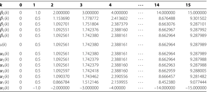
Table 1 Values of successive lower approximationsαn(k) and upper approximationsβn(k), n= 0, 1, 2, 3, 4, 5, 6

k 0 1 2 3 4 ··· 14 15

β0(k) 0 1.0 2.000000 3.000000 4.000000 · · · 14.000000 15.000000

β1(k) 0 0.5 1.153690 1.778772 2.413602 · · · 8.676488 9.301502

β2(k) 0 0.5 1.092701 1.751804 2.387379 · · · 8.663076 9.287101

β3(k) 0 0.5 1.092551 1.742376 2.388160 · · · 8.662967 9.287992

β4(k) 0 0.5 1.092561 1.742380 2.388161 · · · 8.662964 9.287989

u(k) 0 0.5 1.092561 1.742380 2.388161 · · · 8.662964 9.287989

α6(k) 0 0.5 1.092561 1.742380 2.388161 · · · 8.662964 9.287989

α5(k) 0 0.5 1.092561 1.742379 2.388161 · · · 8.662964 9.287988

α4(k) 0 0.5 1.092561 1.742379 2.388160 · · · 8.662963 9.287988

α3(k) 0 0.5 1.092597 1.742418 2.388160 · · · 8.662959 9.288005

α2(k) 0 0.5 1.090370 1.743462 2.390556 · · · 8.666457 9.281482

α1(k) 0 0.5 0.866784 1.512146 2.159955 · · · 8.452380 9.077444

α0(k) 0 –1.0 –2.000000 –3.000000 –4.00000 · · · –14.000000 –15.000000

where Ln– = min{–αn–(), . – αn–()}, Mn– = min{βn–(),βn–() – .}, kn– = min{Ln–,_n–},pn–=min{Mn–,_n–}and

P(k,u) = 

k–

k+_–_max

 – maxs∈Z[k–,k]u(s) k+_–_max

+ 

k–

k+_–_u₍_k₎

 – u(k) k+_–_u₍_k₎

+ 

k–

k+_–_u₍_τ₍_k₎₎

 – u(τ(k)) k+_–_u₍_τ₍_k₎₎

.

IVPs () and () are solved by a computer realization of the algorithm given in Sec-tion , and the results are given in Table . The obtained numerical results demonstrate the rapid monotonic convergence of both sequences.

Competing interests

The authors declare that they have no competing interests.

Authors’ contributions

All authors contributed equally in the preparation of this article. Both authors read and approved the ﬁnal manuscript.

Acknowledgements

Research was partially supported by Fund Scientiﬁc Research MU13FMI002, Plovdiv University.

Received: 29 October 2013 Accepted: 27 January 2014 Published:31 Mar 2014

References

1. Wang, Q, Perc, M, Duan, Z, Chen, G: Delay-induced multiple stochastic resonances on scale-free neuronal networks. Chaos19, 023112 (2009). doi:10.1063/1.3133126

2. Perc, M: Spatial coherence resonance in neuronal media with discrete local dynamics. Chaos Solitons Fractals31, 64-69 (2007)

3. Ferraro, T, de Candia, A, Gamba, A, Coniglio, A: Synchronization transitions on small-world neuronal networks: eﬀects of information transmission delay and rewiring probability. EPL83, 50008 (2008). doi:10.1209/0295-5075/83/50009 4. Wang, Q, Perc, M, Duan, Z, Chen, G: Synchronization transitions on scale-free neuronal networks due to ﬁnite

information transmission delays. Phys. Rev. E80, 026206 (2009)

5. Gelisken, A, Sinar, G, Kurbanli, A: On the asymptotic behavior and periodic nature of a diﬀerence equation with maximum. Comput. Math. Appl.59(2), 898-902 (2010)

6. Touafek, N, Halim, Y: On max type diﬀerence equations: expressions of solutions. Int. J. Nonlinear Sci.11(4), 396-402 (2011)

7. Yang, X, Liao, X, Li, C: On a diﬀerence equation with maximum. Appl. Math. Comput.181(1), 1-5 (2006) 8. Atici, FM, Cabada, A, Ferreiro, J: First order diﬀerence equations with maxima and nonlinear functional boundary

value conditions. J. Diﬀer. Equ. Appl.12(6), 565-576 (2006)

9. Tisdell, C: On first-order discrete boundary value problems. J. Differ. Equ. Appl.12, 1213-1223 (2006) 10. Agarwal, R, Cabada, A, Otero-Espinar, V: Existence and uniqueness results forn-th order nonlinear difference

(14)

11. Jankowski, T: First-order functional diﬀerence equations with nonlinear boundary value problems. Comput. Math. Appl.59, 1937-1943 (2010)

12. Cabada, A: The method of lower and upper solutions for periodic and anti periodic diﬀerence equations. Electron. Trans. Numer. Anal.27, 13-25 (2007)

13. Cabada, A, Otero-Espinar, V, Pouso, V: Existence and approximations of solutions of ﬁrst order discontinuous diﬀerence equations with nonlinear global conditions in the presence of lower and upper solutions. Comput. Math. Appl.39, 21-33 (2000)

14. Hristova, S, Golev, A, Stefanova, K: Quasilinearization of the initial value problem for diﬀerence equations with maxima. J. Appl. Math.2012, Article ID 159031 (2012). doi:10.1155/2012/159031

15. Atici, FM, Cabada, A, Ferreiro, J: Existence and comparison results for first order periodic implicit difference equations with maxima. J. Differ. Equ. Appl.8(4), 357-369 (2002)

16. Agarwal, R, Hristova, S: Quasilinearization for initial value problems involving diﬀerential equations with “maxima”. Math. Comput. Model.55(9-10), 2096-2105 (2012)

17. Bainov, D, Hristova, S: Diﬀerential Equations with Maxima. Taylor & Francis, CRC Press, London (2011) 18. Golev, A, Hrisova, S, Rahnev, A: An algorithm for approximate solving of diﬀerential equations with “maxima”.

Comput. Math. Appl.60, 2771-2778 (2010)

10.1186/1029-242X-2014-132