A Novel TANAN’s Algorithm for Solving Economic Load Dispatch Problems

(1)

ISSN 2250-3153

www.ijsrp.org

A Novel TANAN’s Algorithm for Solving Economic

Load Dispatch Problems

Subramanian R*, Thanushkodi K**

*Associate Professor, Akshaya College of Engineering and Technology, Coimbatore, 642 109, India **Director, Akshaya College of Engineering and Technology, Coimbatore, 642 109, India

Abstract -The Economic Load Dispatch (ELD) problems in

power generation systems is to reduce the fuel cost by reducing the total cost for the generation of electric power. This paper presents a Novel TANAN‘s Algorithm (NTA) for solving ELD Problems. The main objective of NTA is to minimize the total fuel cost of the generating units subjected to limits on generator true power output, power loss. The NTA is a simple numerical random search approach based on a parabolic TANAN function. This paper presents an application of NTA to ELD problems for different IEEE standard test systems. ELD is applied and compared with various optimization techniques and the simulation results show that the proposed algorithm outperforms previous optimization methods.

Index Terms

-

Economic Load dispatch, Evolutionary

Programming (EP), Genetic Algorithm (GA), Particle Swarm Optimization (PSO), Taguchi Method (TM)

NOMENCLATURE

ai, bi, ci : Fuel cost coefficients of i th

generator ($/MW2h, $/MWh, $/h)

Fi : Fuel cost of ith generator, $/h

Ft ; Total fuel cost, $/h

n :Number of generators Pi : Output of ith generator, MW

Pimax : Maximum generation limit of ith generator,

MW

Pimin : Minimum generation limit of ith generator,

MW

Pl : Power loss, MW

Pd : System power demand, MW

B : Loss coefficient matrix

Ti : TANAN Function for ith generator

ri , si , ti : Coefficients of TANAN function for ith

generator

x : TANAN function Variable

I. INTRODUCTION

Electrical power industry restructuring has created highly vibrant and competitive market that altered many aspects of the power industry. In this changed scenario, scarcity of energy resources, increasing power generation cost,

environment concern, ever growing demand for electrical energy necessitate optimal dispatch. Economic Load Dispatch (ELD) is one of the important optimization problems in power systems that have the objective of dividing the power demand among the online generators economically while satisfying various constraints. Since the cost of the power generation is exorbitant, an optimum dispatch saves a considerable amount of money. Optimal generation dispatch is one of the most important problems in power system engineering, being a technique commonly used by operators in every day system operation. Optimal generation seeks to allocate the real and reactive power throughout power system obtaining optimal operating state that reduces cost and improves overall system efficiency. The economic dispatch problem reduces the system cost by allocating the real power among online generating units. In the economic dispatch problem the classical formulation presents deficiencies due to simplicity of models. Here, the power system modelled through the power balance equation and generators are modelled with smooth quadratic cost functions and generator output constraints.

To improve power system studies, new models are continuously being developed that result in a more efficient system operation. Cost functions that consider valve point loadings, fuel switching, and prohibited operating zones as well as constraints that provide more accurate representation of system such as: emission, ramp rate limits, line flow limits, spinning reserve requirement and system voltage profile. The improved models generally increase the level of complexity of the optimization problem due to the non-linearity associated with them.

Traditional algorithms like lambda iteration, base point participation factor, gradient method, and Newton method can solve the ELD problems effectively if and only if the fuel-cost curves of the generating units are piece-wise linear and monotonically increasing. The basic ELD considers the power balance constraint apart from the generating capacity limits. However, a practical ELD must take ramp rate limits, prohibited operating zones, valve point effects, and multi fuel options into consideration to provide the completeness for the ELD formulation. The resulting ELD is a non-convex optimization problem, which is a challenging one and cannot be solved by the traditional methods.

(2)

www.ijsrp.org Algorithms. These algorithms provide an alternative for

obtaining global optimal solutions, especially in the presence of non-continuous, non-convex, highly solution spaces. These algorithms are population based techniques which explore the solution space randomly by using several candidate solutions instead of the single solution estimate used by many classical techniques. The success of evolutionary algorithms lies in the capability of finding solutions with random exploration of the feasible region rather than exploring the complete region. This results in a faster optimization process with lesser computational resources while maintaining the capability of finding global optima. The conventional optimization methods are not able to solve such problems due to local optimum solution convergence. Meta-heuristic optimization techniques especially Genetic Algorithms (GA) [1], Particle Swarm Optimization (PSO) [12] and Differential Evaluation (DE) [7] gained an incredible recognition as the solution algorithm for such type of ELD problems in last decade.

II. PROBLEM FORMULATION

The classical ELD problem is an optimization problem that determines the power output of each online generator that will result in a least cost system operating state. The objective of the classical economic dispatch is to minimize the total system cost where the total system cost is a function composed by the sum of the cost functions of each generator. This power allocation is done considering system balance between generation and loads, and feasible regions of operation for each generating unit.

The objective of the classical ELD is to minimize the total fuel cost by adjusting the power output of each of the generators connected to the grid. The total fuel cost is modelled as the sum of the cost function of each generator.

The basic economic dispatch problem can be described mathematically as a minimization of problem.

Minimize Ft = (1) Where Fi (Pi ) is the fuel cost equation of the

‗i‘th plant. It is the variation of fuel cost in $ with generated Power (MW).

(2)

The total fuel cost to be minimized is subject to the following constraints.

(3)

(4)

(5)

IV. NOVEL TANAN’s ALGORITHM

The Novel TANAN‘s Algorithm (NTA) is specially defined for solving economic dispatch problems. The algorithm is stated as follows. The TANAN function is given by

(7)

with a power balance constraint

Where

Ti - TANAN function

ri, si & ti - coefficients of TANAN function

x - TANAN function variable

The coefficients ri, si and ti has been selected y taking

the minimum limits of ith generator respectively. The TANAN function variable ‗x‘ is a random variable and it ranges from 0 to 2.The value of ‗x‘has been selected by maximum of twenty random trial runs between 0 to 2 (tested for all IEEE standard test systems) with an increment of 0.1 and the value corresponds to minimum fuel cost has been taken from the random trials and its value is again fine-tuned by several trial runs to get the optimum value of fuel cost. Each generator is assigned by individual TANAN function and the value of each TANAN function is considered as the power output of that particular generator(Ti= Pi).Since the TANAN function is a

parabolic function , it has an extreme lowest point that corresponds to the optimum value of fuel cost.

A. Algorithm:

Step1:Assign TANAN function to each

generators.

Step2:Initialize ri, si and ti values.

Step3:Assign the value of x by several trial runs.

Step4: Assign Ti = Pi.

Step5:If Pi ≤ Pimin then fix Pi = Pimin and

if Pi ≥ Pimax then fix Pi = Pimax. Step6:Verify Pd and generator limits lie

within the given range, if not adjust the value of x to meet the power balance.

Step7:Notify the fuel cost values

and stop the process.

(3)

ISSN 2250-3153

www.ijsrp.org

V. SIMULATION RESULTS

[image:3.595.40.247.55.408.2]

The NTA for ELD problem have implemented in MATLAB and it was run on a computer with Intel Core2 Duo processor, 3GB RAM memory and Windows XP operating system. Since the performance of the proposed algorithm sometimes depends on input parameters, they should be carefully chosen. After several runs, the following results were obtained and are tabulated.

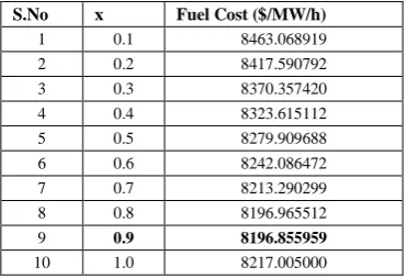
Table 1- Results of IEEE- 3 machine (Pd= 850 MW) test system without considering the power loss for different ‗x‘

values by NTA.

S.No x Fuel Cost ($/MW/h)

1 0.1 8463.068919

2 0.2 8417.590792

3 0.3 8370.357420

4 0.4 8323.615112

5 0.5 8279.909688

6 0.6 8242.086472

7 0.7 8213.290299

8 0.8 8196.965512

9 0.9 8196.855959

10 1.0 8217.005000

From the table 1, the value of‘ x‘ lies in the range of 0.8 to 0.9 for the minimum fuel cost and to meet the power

[image:3.595.335.527.140.223.2]

demand and the optimum value of x is again fine tuned by several random trials and the optimum value for minimum fuel cost obtained at x=0.8515 as shown in table 2.

Table 2- Best result from IEEE- 3 machine test system (Pd = 850 MW) without considering the Power loss

(x = 0.8515)

Description NTA

P1(MW) 386.482838 P2(MW) 334.689550 P3(MW) 128.827613 Total power(MW) 850.000000 Total fuel cost($/MW/h) 8194.636018

[image:3.595.325.542.278.427.2]

Execution time(sec) 0.001474

Table 3-Results from IEEE-6 machine (Pd=1263MW) test system including power loss for different ‗x‘ values by NTA.

S.No x Total cost ($/MW/h)

1 0.1 17655.684680

2 0.2 17345.865169

3 0.3 17017.906250

4 0.4 16684.352690

5 0.5 16359.349516

6 0.6 16058.615066

7 0.7 15799.410956

8 0.8 15602.409125

9 0.9 15480.812974

10 1.0 15430.182993

11 1.1 15447.425273

12 1.2 15534.553158

From the table 3, the value of‘ x‘ lies in the range of 1.0 to 1.1 for the minimum fuel cost and to meet the power balance and the optimum value of x is again fine tuned by several random trials and the optimum value for minimum fuel cost obtained at x=1.03 as shown in table 4.

Table 4 -Best result of IEEE- 6 machine (Pd=1263MW) test system including power loss (x=1.03)

P1(MW) 446.420479

P2(MW) 154.545000

P3(MW) 247.272000

P4(MW) 150.000000

P5(MW) 154.545000

P6(MW) 120.000000

Total power (MW) 1272.782479 Total fuel cost ($/MW/h) 15428.730294 Power loss (MW) 9.782479

CPU time (sec) 0.254221

Table 5- Results from IEEE-6 machine (Pd=283.4MW) test system including power loss for different ‗x‘ values by NTA.

1 0.1 977.218838

[image:3.595.327.538.538.668.2] [image:3.595.71.257.586.712.2]

(4)

www.ijsrp.org

3 0.3 976.117638

4 0.4 979.222847

5 0.5 986.062392

6 0.6 997.753602

7 0.7 1015.528440

8 0.8 1040.732620

9 0.9 1074.824641

10 1.0 1119.374738

[image:4.595.324.540.49.186.2]

Table 6-Best result of IEEE- 6 machine (Pd=283.4MW) test system including power loss (x=0.235)

P1(MW) 197.352501

P2(MW) 25.804500

P3(MW) 19.353375

P4(MW) 12.902250

P5(MW) 12.902250

P6(MW) 15.482700

Total power (MW) 283.797576 Total fuel cost ($/MW/h) 975.622401 Power loss (MW) 0.397576

[image:4.595.55.274.49.142.2]

CPU time (sec) 0.003089

Table 7- Results from IEEE-15 machine (Pd=2640 MW) test system including power loss for different ‗x‘ values by NTA.

1 0.1 33386.921422

2 0.2 33333.759960

3 0.3 33284.089414

4 0.4 33242.851931

5 0.5 33215.609374

6 0.6 33208.528755

7 0.7 33228.366041

8 0.8 33282.448369

9 0.9 33378.654686

10 1.0 33525.394866

[image:4.595.324.541.242.373.2]

Table 8 -Best result of IEEE- 15 machine (Pd=2640 MW) test system including power loss (x=0.747)

P1(MW) 448.431247

P2(MW) 410.292150

P3(MW) 54.705620

P4(MW) 54.705620

P5(MW) 410.292150

P6(MW) 369.262935

P7(MW) 369.262935

P8(MW) 164.116860

P9(MW) 68.382025

P10(MW) 68.382025

P11(MW) 54.705620

P12(MW) 54.705620

P13(MW) 68.382025

P14(MW) 41.029215

P15(MW) 41.029215

Total power (MW) 2677.685262 Total fuel cost ($/MW/h) 33389.662792

Power loss (MW) 37.685262 CPU time (sec) 0.007171

Table 9- Results from IEEE-20 machine (Pd=2500 MW) test system including power loss for different ‗x‘ values by NTA.

1 0.1 61355.381113

2 0.2 61295.578628

3 0.3 61271.142479

4 0.4 61300.750489

5 0.5 61405.293039

6 0.6 61607.772058

7 0.7 61933.190026

8 0.8 62408.429576

9 0.9 63062.124409

10 1.0 63906.958143

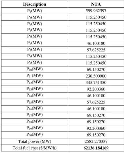
[image:4.595.55.274.424.551.2]

Table 10-Best result of IEEE- 15 machine (Pd=2500 MW) test system including power loss (x=0.747)

P1(MW) 599.962597

P2(MW) 115.250450

P3(MW) 115.250450

P4(MW) 115.250450

P5(MW) 115.250450

P6(MW) 46.100180

P7(MW) 57.625225

P8(MW) 115.250450

P9(MW) 115.250450

P10(MW) 69.150270

P11(MW) 230.500900

P12(MW) 345.751350

P13(MW) 92.200360

P14(MW) 46.100180

P15(MW) 57.625225

P16(MW) 46.100180

P17(MW) 69.150270

P18(MW) 69.150270

P19(MW) 92.200360

P20(MW) 69.150270

[image:4.595.324.538.484.748.2]

(5)

ISSN 2250-3153

www.ijsrp.org

[image:5.595.25.270.150.491.2]

Power loss 798(MW) 82.270337 CPU time (sec) 0.009748

Table 11 - Comparison Table Showing Simulation Result of

NTA for IEEE 3-unit test system (Pd=850 MW) with valve point loading effect along with GA [1], PSO [9],DE[9],NPSO-

[image:5.595.36.276.541.706.2]

LRS[8],BFO[9]and BBO [9] Algorithms.

Fig-4 Comparison chart for IEEE-6 machine test system outputs (Pd=1263MW) with power loss.

Fig-5 Comparison chart for fuel cost for IEEE-6 machine test system (Pd=1263MW) with power loss.

VI. CONCLUSION

The proposed NTA to solve ELD problem with the practical constraints has been presented in this paper. From the comparison table it is observed that the proposed algorithm exhibits a comparative performance with respect to other population based techniques. It is clear that the NTA is a simple numerical random search technique for solving ELD problems. From the simulations, it can be seen that NTA gave the best result of minimized fuel cost, reduced power loss and very less computational time compared to all other optimization methods. In future, the proposed NTA can be used to solve ELD considering ramp rate limits and prohibited operating zones and also for finding the optimal value of the NTA variable ‗x‘ by developing standard search techniques.

References

[1] D. C. Walters and G. B. Sheble, Genetic Algorithm Solution of Economic Dispatch with Valve Point Loading, IEEE Transactions on Power Systems,Vol. 8, No.3,pp.1325–1332, Aug. 1993.

[2] P. H. Chen and H.C. Chang, Large-Scale Economic Dispatch by Genetic Algorithm, IEEE Transactions on Power Systems, Vol. 10, No.4,pp. 1919–1926, Nov. 1995.

[3] D. Simon, ―Biogeography-based optimization,‖ IEEE Trans. Evol. Comput., vol. 12, no. 6, pp.702–713, Dec. 2008.

[4] G. B. Sheble and K. Brittig, ―Refined genetic algorithm- economic dispatch example‖, IEEE Trans. Power Systems, Vol.10, pp.117-124, Feb.1995.

[5] B. K. Panigrahi, V. R. Pandi. ―Bacterial foraging optimization: Nelder-Mead hybrid algorithm for economic load dispatch.‖ IET Gener. Transm, Distrib. Vol. 2, No. 4. Pp.556-565, 2008.

[6] Dervis Karaboga and Bahriye Basturk, ‗Artificial Bee Colony (ABC) Optimization Algorithm for Solving Constrained Optimization Problems,‘ Springer-Verlag, IFSA 2007, LNAI 4529, pp. 789–798. [7] R. Storn and K. Price, Differential Evolution—A Simple and Efficient

Adaptive Scheme for Global Optimization Over Continuous Spaces, International Computer Science Institute,, Berkeley, CA, 1995, Tech. Rep. TR-95–012.

[8] Selvakumar I.A, Thanushkodi K, ―A new particle swarm optimization solution to non convex economic load dispatch problems‖, IEEE Transactions on Power Systems; 22:1.

[9] Mohammad Moradi-Dalvand∗, Behnam Mohammadi-Ivatloo, Arsalan Najafi, Abbas Rabiee Erratum to ―Continuous quick group search optimizer for solving non-convex economic dispatch problems‖Electr. Power Syst. Res. 93 (2012) 93–105.

[10] Jong-Bae Park, Member, IEEE, Ki-Song Lee, Joong-Rin Shin, and Kwang Y. Lee, Fellow, IEEE “A Particle Swarm Optimization for Economic Dispatch With Non smooth Cost Functions‖, IEEE transactions on power systems, vol. 20, no. 1, February 2005

[11] Derong Liu, Fellow, IEEE, and Ying Cai, Student Member, IEEE “Taguchi Method for Solving the Economic Dispatch Problem With Non smooth Cost Functions‖, IEEE transactions on power systems, vol. 20, no. 4, November 2005

[12] G. Zwe-Lee, "Particle swarm optimization to solving the economic dispatch considering the generator constraints," IEEE Transactions on Power Systems, vol. 18, pp. 1187-1195, 2003

(6)

www.ijsrp.org problem with ramp rate limit and prohibited operating zones‖,IEEE word

congress on Nature and Biologically inspired computing (NaBIC)-2009, pp- 1237 – 1242 .

[14] A. Bakirtzis, V. Petridis, and S. Kazarlis, ―Genetic Algorithm Solution to the Economic Dispatch Problem‖, Proceedings. Inst. Elect. Eng. –Generation, Transmission Distribution, Vol. 141, No. 4, pp. 377– 382, July 1994.

[15] E. Zitzler, M. Laumanns, and S. Bleuler, ―A Tutorial on Evolutionary Multi-objective Optimization,‖ Swiss Federal Institute of Technology _ETH_ Zurich, Computer Engineering and Networks Laboratory _TIK_, Zurich, Switzerland.

[16] J. Sun, W. Fang, D. Wang, and W. Xu, "Solving the economic dispatch problem with a modified quantum-behaved particle swarm optimization method," Energy Conversion and Management, vol. 50, pp. 2967-2975, 2009.

[17] A. J. Wood and B. F. Wollenberg, ―Power Generation Operation and Control,‖ 2nd Edition, Wiley, New York, 1996.

[18] A. Chakrabarti and S. Halder, ―Power System Analysis Operation and Control,‖ 3rd Edition, PHI, New Delhi, 2010

R. Subramanian received the B.E degree in Electrical and Electronics Engineering from Coimbatore Institute of Technology in the year 2005 and M.E degree in Power Systems Engineering from Government College of Technology, Coimbatore in the year 2007. He is currently doing PhD in the area of Power system control and operation under Anna University. Presently he is working as an Associate professor in the Department of Electrical and Electronics Engineering at Akshaya College of Engineering and Technology, Coimbatore. His research interests are power system analysis, power system control and operation, mathematical computations, optimization and Soft Computing Techniques.