A Novel Fast Algorithm for Exon Prediction in Eukaryotic Genes using Linear Predictive Coding Model and Goertzel Algorithm based on the Z Curve

(1)

A Novel Fast Algorithm for Exon Prediction in

Eukaryotic Genes using Linear Predictive Coding Model

and Goertzel Algorithm based on the Z-Curve

Hamidreza Saberkari, Mousa Shamsi, Hamed Heravi, Mohammad Hossein Sedaaghi

Faculty of Electrical Engineering, Sahand University of Technology, Tabriz, Iran.

ABSTRACT

Punctual identification of protein-coding regions in Deoxyribonucleic Acid (DNA) sequences because of their 3-base periodicity has been a challenging issue in bioinformatics. Many DSP (Digital Signal Processing) techniques have been applied for identification task and concentrated on assigning numerical values to the symbolic DNA sequence and then applying spectral analysis tools such as the short-time discrete Fourier transform (ST-DFT) to locate periodicity components. In this paper, first, the symbolic DNA sequences are converted to digital signal using the Z-curve method, which is a unique 3-D plot to illustrate DNA sequence and presents the biological behavior of DNA sequence. Then a novel fast algorithm is proposed to investigate the location of exons in DNA strand based on the combination of Linear Predictive Coding Model (LPCM) and Goertzel algorithm. The proposed algorithm leads to increase the speed of process and therefor reduce the computational complexity. Detection of small size exons in DNA sequences, exactly, is another advantage of our algorithm. The proposed algorithm ability in exon prediction is compared with several existing methods at the nucleotide level using: (i) specificity - sensitivity values; (ii) Receiver Operating Curves (ROC); and (iii) area under ROC curve. Simulation results show that our algorithm increases the accuracy of exon detection relative to other methods for exon prediction. In this paper, we have also developed a useful user friendly package to analyze DNA sequences.

Keywords

DNA sequence; Protein coding regions; Signal processing; Exon; Linear predictive coding model; Goertzel algorithm.

1. INTRODUCTION

Deoxyribonucleic acid (DNA) is of the most important chemical compounds in living cells, bacteria and some viruses [1]. A sequence of DNA is a long molecule of biopolymer origin which carries the genetic information and has the ability of expression and replication. It consists of two strands of linear polymers, each made of monomer nucleotide units. Figure 1 shows the DNA molecule structure [2]. Each nucleotide is made of three chemical components: a sugar (deoxyribose), a phosphate group, and a nitrogenous base. There are four possible bases: Adenine and guanine which are purines and have bicyclic structures, and cytosine and thymine which are pyrimidines, and have monocyclic structures. The nucleotides, based on containing bases, are often abbreviated as A, G, C, and T, respectively.

In eukaryotic cells, the DNA is divided into genes and inter-genic spaces. Only genes are responsible for protein synthesis. The information encoded in the genes, is copied to a molecule called messenger RNA (mRNA). This process is called transcription. The next step is called translation which

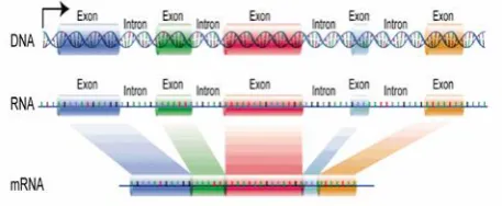
converts mRNA into chains of linked amino acids called polypeptides. Proteins consist of a single type of polypeptides or combinations of different types. Every three nucleotide combination is called a codon. Each codon specifies one amino acid, so sequences of codons in mRNA determine specific polypeptide chains. Each gene consists of exon and intron regions (Figure 2). In transcription of eukaryotic DNA into mRNA, introns are omitted (spliced away) and only exons are translated into proteins. Therefore, exons are called protein-coding regions because they carry the necessary information for protein coding [3-5]. The proteins are the machinery of the cell and determine its properties, so detection of protein-coding regions is very important in understanding of biological functions. Protein-coding regions exhibit a period-3 behavior that is not found in other parts of the DNA and this property can be used in digital processing methods for gene detection and exon prediction purposes [6].

The attendance of long-range correlation which is considered as the background noise results in more difficulty of exon finding in DNA sequences [7-8]. Also because of the complex nature of the gene identification problem, we usually need a more efficient model that can effectively represent the characteristics of protein-coding regions. Up to now, distinctive methods have been proposed to overcome these problems which in a comprehensive categorization they can be divided into two groups; Model-dependent or supervised methods and Model-independent or Filter-based methods. Model-dependent methods like Hidden Markov Model (HMM) [9], neural network [10] and pattern recognition [11], are based on some former information gathered from the available datasets, and have been successfully used to predict exons in genes. In [9] an HMM model is proposed for gene identification which resolves three basic problems; Evaluation, Decoding and Learning problems, which can be solved using Forward and Backward, Viterbi and Baum-Welch algorithms, respectively. In [10] by introducing two new methods, one-vs-others and all-vs-all methods, and using Support Vector Machine (SVM) and Neural Network (NN) methods as base classifiers, protein fold recognition has been done.

(2)

Notch filter with the central frequency of 2π/3 in order to remove the background noise. In [15], first, the numerical DNA sequence is passed through a notch filter and then a sliding windowed Discrete Fourier Transform (DFT) is applied on the filtered sequence. In [16] a windowless technique based on the Z-curve has been proposed to identify gene islands in total DNA sequence which called cumulative GC-Profile method. The main characteristic of the proposed method in [16] is that the resolution of the algorithm output in displaying the genomic GC content is high since no sliding window is used, but the computational complexity of this method is also high. In [17] an appropriate method is proposed to predict the protein regions by combining the DFT and Continues Wavelet Transform (CWT). CWT leads to eliminate the high frequency noise and therefore improves the accuracy of the prediction. In [18] a new algorithm is proposed based on Fourier Transform using Bartlett window to suppress the non-exonic regions. Authors in [19] used time domain algorithms to determine the coding regions in DNA sequences. Adaptive filters [20] are one of the best tools for prediction tasks. In [21-22] authors proposed two adaptive filtering approaches based on Kalman filter and Least Mean Squares (LMS). However, the major problem with LMS is that the convergence behavior of the algorithm is slow which leads to high computational complexity. In [23] a parametric method based on autoregressive (AR) model is proposed for spectral estimation. The AR model has the advantage over the DFT that they work with smaller window sizes and, thus, shorter sequences. Using the fixed-length window is the major restriction of discussed filter-based algorithms. In many cases, size of the selected window is not successful to predict the small size coding regions. So these methods have no sensitivity to determine the protein coding regions, especially small size of exon regions. Also the run process in the mentioned algorithms is high, so there is a demand for presenting a fast and efficient method to overcome these limitations.

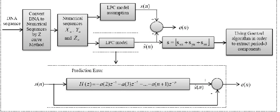
[image:2.595.349.485.76.241.2]

In this paper, a fast model-independent method based on a Liner Predictive Coding (LPCM) and Goertzel algorithm is proposed to identify the exon regions based on period-3 property in DNA sequences. First, the symbolic DNA sequence is converted into the numerical values by the Z-curve method. Then an appropriate model which named Linear Predictive Coding Model (LPCM) has been provided to remove the redundancy information in numerical DNA signal (i.e., high frequency noise components). Finally the Goertzel algorithm is applied to the estimated sequence in order to extract the period-3 components. Compared with the other existed techniques, increasing the speed of process and reducing the computational complexity are the major advantages of our proposed algorithm. Also the amount of background noise is greatly reduced in our method and the protein coding regions with small sizes are well recognized. The rest of the paper is organized as follows: In section 2 the proposed algorithm is described in details. The evaluation criteria at nucleonic level are expressed in section 3. Simulation results using Genbank database are reported in section 4. Finally, conclusion is mentioned in section 5.

Fig 1: DNA molecule structure.

Fig 2: Exon/Intron regions for eukaryotic DNA.

2. PROPOSED ALGORITHM

Figure 3 shows the block diagram of our proposed algorithm to identify protein coding regions. The main steps of the algorithm are as follows that will be discussed in more details in this section.

- Mapping of DNA sequence to the numerical form using the Z-curve method,

- Using Linear Predictive Coding Model (LPCM) to remove the noise from the numerical sequence and achieve an appropriate model of numerical sequence,

- Using Goertzel algorithm to extract the period-3 components.

2.1 DNA numerical representation

Converting the DNA sequences into digital signals [24, 25] opens the possibility to apply signal processing methods for analyzing of genomic data and reveals features of chromosomes. The genomic signal approach has already proven its potential in revealing large scale features of DNA

sequences maintained over distance of

10

6



10

8base pairs, including both coding and non-coding regions, at the scale of whole genomes or chromosomes [26-28].

[image:2.595.317.546.289.383.2]

(3)

representation is used to map DNA character string into numerical sequence. Based on this curve, each DNA sequence could be described separately by three independent

distributions

X

_n,

Y

_n and

Z

_n, which each of these distributions is as follows [30]:



 





 









i i

 

i i



i

i i i i i i i i

i i i i i

C G T A z

i z

y x T G C A y

T C G A x

   

   

  

   

3 , 2 , 1 , 1 , 1 ,

, ₍₁₎

where

A

_i,

C

_i,

G

_i, and

T

_i are the cumulative numbers of the bases A, C, G and T, respectively, occurring in the

sub-sequence from the first to the

n

thbase in the DNA sequence. We define

A

₀



C

₀



G

₀



T

₀



0

. Each of these components has a biological interpretation. The first

sequence

X

_n indicates the existence of either A or G which represents a differentiation between the purines/pyrimidine (R/Y) bases along the DNA strand. Similarly, the second

sequence

Y

_n represents the distribution of the amino/keto

(M/K) types bases along the DNA sequence while the third

sequence

Z

_n represents the distribution of the strong/weak

hydrogen bonds (S/W). For the sub-sequence which made of

thefirst base to the

n

thbase of DNA sequence, when purine bases (A or G) are more than pyrimidine ones (C or T)

then

X

_n > 0 and if not

X

_n < 0. When the amounts of purines and pyrimidine bases are equal then

X

_n= 0. Similarly when Amino bases (A or G) are more than keto

bases (C or T) then

Y

_n> 0 and if not

Y

_n< 0 and if these bases

are equal then

Y

_n = 0 and finally when strong hydrogen

linkage bases (A or T) are more than weak hydrogen linkage

bases (G or C)

Z

_n> 0 and if not

Z

_n< 0 and in case amounts

of these bases are equal then

Z

_n=0. Therefore Z curve

includes all these data that has a DNA sequence adapted to itself [31].

2.2 Linear Predictive Coding Model

Linear Predictive Coding Model [32] is one of the more efficient techniques for analyzing of non-stationary signals. The importance of this method lies to its ability to provide extremely accurate estimates of the signal parameters, and in its relative speed of computation. The main idea of this model is that a signal sample can be estimated as a linear combination of its previous samples. By minimizing the sum of the squared error between the actual signal samples and the estimated ones, a set of estimated coefficients can be calculated.

Let

s(n),

n



1,

2,

..,

N

be a protein sequence with length N whose elements are represented the Z-curve values for the corresponding amino acids. The estimated Z-curve value of each amino acid at position n is shown by

s

ˆ

(

n

)

and it can be calculated as a linear combination of p previous Z-curve values as follows:









p

1 k

k

s(n

k)

a

(n)

s

ˆ

(2)

where

 

a

_k are called the linear prediction coefficients. In this paper, the value of p is chosen 6.

The prediction error e(n) between the observed Z-curve value s(n) and the estimated Z-curve value

s

ˆ

(

n

)

is defined:













p

1 k

k

s(n

k)

a

s(n)

(n)

s

s(n)

e(n)

ˆ

(3)

The estimated coefficients

 

a

_k can be efficiently

[image:3.595.61.542.318.510.2]

determined by minimizing the sum of squared error as follows:

(4)

28 ] [n x ] [n

x

y

k

[

n

]

[

n

x

y

_k

[

n

]

2 N 1 n N 1 n p 1 k k 2

k)

s(n

a

s(n)

(n)

e

E



  

















(4)

To solve Eq. (4), we differentiate E with respect to each

a

_k

and equate result to zero:

p.

...,

1,

k

,

0 a

E

k





(5)

By solving Eq. (5), a set of p linear equations is obtained as follows:







p 1 k

k

r(m

k)

r(m)

,

m

1,

...,

p

a

(6)

in which, r(m) is the autocorrelation of s(n), that is:









N 1 n

m)

s(n

s(n)

r(m)

(7)

The matrix form of Eq. (6) can be expressed as:

r

Ra



(8)

where R is a p×p autocorrelation matrix, r is a p×1 autocorrelation vector, and a is a p×1 vector of prediction coefficients. So, the three parameters R, r and a are defined as follows:                                    ) ( 0 . . . 0 . . . . . . . . . . . . . . ) 2 ( . ) ( 0 ) 1 ( . . ) ( 0 . . . . . . . . . . . . . ) 2 ( . . . ) 1 ( ) 2 ( 0 . . . 0 ) 1 ( p r r p r r p r r r r r R , ) 1 ( . . ) 2 ( 1 ,                   p a a a                  0 . . 0 1 r (9)

2.3 Goertzel algorithm

In order to apply the Goertzel algorithm, Blackman window is used to segment the estimated sequence from LPC model. The impulse response of the FIR windows has been discussed in [33]. According to [33], Blackman window has the highest amount of attenuation between the other windows. So the background noise is more suppressed by Blackman. The Goertzel algorithm is a digital signal processing technique which provides a means for efficient evaluation of individual terms of the Discrete Fourier Transform (DFT), thus results in useful certain practical application, such as dual-tone multi frequency (DTMF) signals [34], digital multi frequency (MF) receiver [35] and in a very small aperture terminal (VSAT) satellite communication system [36]. In order to express the functionality of this algorithm, it must be noted that the DFT can be formulated in terms of a convolution as follow:











x[n] W u[n]



W x[n] W x[r] 1 W , W x[n] e W , W x[n] [k] X nk N nk N 1 N 0 r r) k(N N kN N 1 N 0 n n) k(N N 1 N 0 n nk N 2π j N nk N                       



(10)

Processing of the signal x[n] through an LTI filter with

impulse response

h

[

n

]

W

Nnk

u

[

n

]





and evaluating the result,

y

_k

[

n

]

at n=N will give the corresponding N-point DFT coefficient

X

[

k

]



y

_k

[

N

]

. This LTI filtering process is illustrated as follows:

Based on the Z-transform of the filter, we have:

    1 k N 1 k N 0 0 N 1 k N 1 m 0 m k 1 m N m 0 m m N m 0 m m N 1 k N 1 k N m 0 m m N z W 1 1 z W 1 z W z W 1 z Wk z Wk z Wk z W 1 z W 1 z Wk H(z)                                       



(11)

The filtering operation can be equivalently performed by the system: Note that: 2 1 1 k N 1 k N 1 k N 1 k N 1 k N z z N 2kπ 2cos 1 z W 1 z W 1 1 . z W 1 z W 1 z W 1 1 H(z)                          (12)

So, the filtering operation can also be equivalently performed by:

u[n]

W

h[n]

nk N 



y

[n]

x[n]



W

nk

u[n]



N k 





m 0 m mk N

z

W

   



]

[

n

x

y

_k

[

n

]

(5)

Hence, as can be seen from Figure 4, the Goertzel filter is composed of a recursive part and a non-recursive part. The DFT coefficients are obtained as the output of the system after N iterations. The recursive part is a second-order IIR filter (resonator) with a direct form structure. The resonant frequency of the first stage filter is set at equally spaced frequency points; that is,

N k

k



 2 (This value is chosen

3 2 _in

our work to extract the period-3 components). The second stage filter can be observed to be an FIR filter, since its calculations do not use of the previous values of the output. In fact, we only compute the recursive part of the filter at each sample and the non-recursive part is computed only after the Nth time instant when the Fourier coefficients are to be determined.

The major advantage of Goertzel algorithm is its ability to reduce the computational complexity relative to other existence methods such as DFT. This algorithm requires N real multiplications and a single complex multiplication to compute X[k] for a given k. However, DFT and decimation in

[image:5.595.304.546.307.407.2]

time FFT require

N

2and N

log

₂

N

complex multiplications to compute X[k], respectively [33].

Fig 4: Filter realization of the Goertzel algorithm [33].

3. Evaluation criteria at nucleotide level

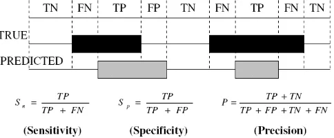
In order to compare accuracy of the different methods for protein coding regions detection the evaluation is done at nucleotide level. For this purpose, we introduce some parameters that are listed as follows:

Sensitivity and Specificity: Figure 5 shows these parameters definition, where true positive (TP) is the number of coding nucleotides correctly predicted as coding, false negative (FN) is the number of coding nucleotides predicted as non-coding. Similarly, true negative (TN) is the number of non-coding nucleotides correctly predicted as non-coding, and false positive (FP) is the number of non-coding nucleotides predicted as coding. By definition of these four quantities, the

parameters sensitivity (

S

_n) and specificity (

S

_p) and precision (P) are defined as follows [37]:

FN TN FP TP

TN TP P

FP TP

TP S

FN TP

TP S

p n

  

 

(13)

Receiver Operating Characteristic (ROC) curves: The receiver operating characteristic (ROC) curves were developed in the 1950s as a tool for evaluating prediction

techniques based on their performance [38]. An ROC curve explores the effects on TP and FP as the position of an arbitrary decision threshold is varied. The ROC curve can be approximated using an exponential model as follow [39]:







β1 x β2x



e

1 α

y





  (14)

in which, parameters



,



₁and



₂can be determined by minimizing the error function:













2









_





n

1 i

i x β x β

y

e

1 α

E(p)

1 i 2 i ₍₁₅₎

where

p









₁



₂



Tand



x

_i

,

y

_i



are points in the ROC plane.

Area under the ROC curve (AUC): This parameter is also a good indicator of the overall performance of an exon-location technique. The greater the AUC leads to the better performance of the tested algorithm [37].

Fig 5: Parameters for evaluation of the accuracy of the algorithms.

4. Simulation Results

In order to demonstrate the performance of the discussed methods, the proposed algorithm is applied on four gene; F56F11.4, AF009962, AF019074 and AJ223321 from Genbank dataset [40]. The gene sequence F56F11.4 (GenBank No. AF099922) is on chromosome III of Caenorhabditis elegans. C elegans is a free living nematode, about 1mm in length, which lives in temperate soil environment. It has five distinct exons, relative to nucleotide position 7021 according to the NCBI database. These regions are 3156-3267, 4756-5085, 6342-6605, 7693-7872 and 9483-9833. AF009962 is the accession number for single exon which has one coding region at position 3934-4581. The gene sequence AF019074 has the length of 6350 which has three distinct exons, 3101-3187, 3761-4574, and 5832-6007. AJ223321 is in the HMR195 dataset. This dataset consists of 195 mammalian sequences with exactly one complete either single-exon or multi-exon gene. All sequences contain exactly one gene which starts with the 'ATG' initial codon and end with a stop codon (TAA, TAG, or TGA). There is one coding region existed in AJ223321 gene sequence which its location is 1196-2764. All mentioned sequences are converted to numerical sequences using Z-curve method.

[image:5.595.67.257.332.444.2]

(6)

After Projection

TP

FP

FP FP

TN Decision

Threshold is 0.161

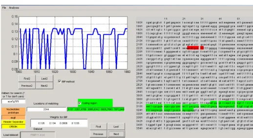
sequences. The graphic display allows the user to view the structure record either as a graphic or as a text record in txt formats. Also it can be useful to search option for special patterns in the sequences (for example, start and stop codons in DNA sequences). The DSP tools are applying to DNA sequences in order to spectral analysis.

Briefly, there are some advantages for this tool as mentioned below:

- Loading of any DNA sequences,

- Genomic sequence representation,

- Conversion of the genomic sequence into digital values by EIIP, binary methods and z-curve,

- Search option for special patterns in the sequence,

- Applying of DSP and non-DSP methods such as DFT on the signal, and

[image:6.595.362.503.73.375.2]

- Prediction of the protein coding regions.

Fig 6: A view of the designed user friendly package for analyzing of the DNA sequence.

Figure 7 (a) shows the Z curve for a sample gene sequence (F56F11.4). As we can observe, it is hard to display such a long character-based sequence on computer screen. Even though the display is made possible, the extraction of any feature from the sequence is still difficult. By applying the Z curve for visualize this sequence; some features of global and local nucleotide composition of a genome can be displayed in a perceivable form. Although the screen resolution in insufficient to convey the details of the curve and help a user to display local features of the Z curve involved at single nucleotide level. To provide more detailed information than the original Z curve, three 1-D projection curves are determined. Figure 7 (b) shows three 1-D curves, which are obtained by projecting the Z curve onto x, y and z axes, respectively.

In this paper, to compare the performance of the proposed algorithm and other tested methods, we use the

[image:6.595.294.542.108.744.2]

parameters

S

_n,

S

_p and P which were described in section 3. Amounts of these parameters achieved from equations (13). The amounts of TP, FP, TN and FN are calculated by changing threshold level in range of 0 and 1 with small steps according Figure 8 (In this figure the value of threshold is 0.161). It can be observed in Figure 8 that if the decision threshold is very high, then there will be almost no false positives, but it won’t be really identified many true positives either.

Fig 7: Z-curve representation for gene sequence F56F11.4. (a) 3-D Z curve (b) Projection curves of the

original Z curve onto x, y and z axes, respectively.

2000 4000 6000 8000 -35

-30 -25 -20 -15 -10 -5 0

X

Y

X-vector Y-vector Z-vector

[image:6.595.40.299.282.423.2]

(b) (a)

Fig 8. Parameters for exon-intron separation problem.

0 1000 2000 3000 4000 5000 6000 7000 8000 9000 10000 0

0.2 0.4 0.6 0.8 1

Sequence index (bp)

Feat

u

re

v

al

u

es

[image:6.595.300.549.415.748.2]

(7)

0 1000 2000 3000 4000 5000 6000 7000 8000 9000 10000 0

0.2 0.4 0.6 0.8 1

Relative base location, n

Peri

o

d

-3

Po

w

er

Sp

ect

ru

m

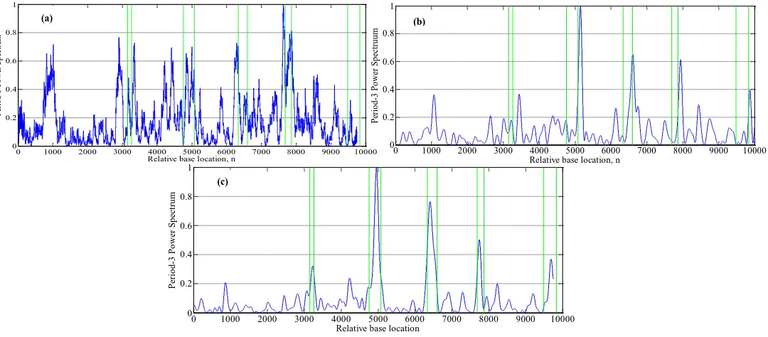
In this paper, to evaluate the performance of the proposed algorithm, the DFT [14] and Multi-Stage filter (MS) [41] methods are implemented. Figures 9-12 (a) and (b) show results of implementation of these methods and the proposed algorithm in identifying protein coding regions in four gene sequences explained above. As can be seen, accuracy of the DFT method for protein coding regions estimation is not high due to the noise associated with the original signal. However, the MS filter resulted a good spectral component compared to DFT and reduced the computational complexity. Also the non-coding regions are relatively suppressed in it, but this method cannot recognize the small size exonic regions. As shown in Figures 9-12 (c), the large amount of noise is removed in the proposed method due to applying the LPC model, and small size exons (For example, first exon in F56F11.4 gene sequence) can be identified because of using the Goertzel algorithm.

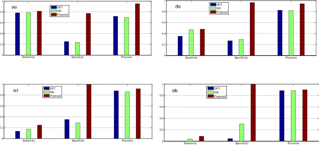
Figures 13 to 16 show the bar chart of sensitivity, specificity and precision in the proposed algorithm and other methods in different thresholds (from Th=0.2 to Th=0.8). As can be seen, the proposed algorithm yields the highest of these values in all threshold levels. By way of illustration, at Th=0.2, this algorithm exhibits relative improvements of 40% and 87% over DFT and MS filter in the Sensitivity in a typical gene

sequence F56F11.4, respectively. Also the parameter

S

_p is improved by the factors of 3.1 and 5.7 relative to the DFT and MS filter in the sequence, respectively. Finally, the proposed algorithm shows relative improvements of 15% and 33% over the MS filter and DFT methods, respectively, in terms of Precision measure. Similar results of the proposed algorithm are apparent for the other gene sequences as shown in Figures 14-16.

In Table I, the number of false positive nucleotides, specificity and precision for specified sensitivities are

presented for the proposed and the other tested methods. According to this table, the proposed algorithm has the minimum nucleotides incorrectly identified as exons in all four gene sequences. For example in F56F11.4, at the sensitivity of 0.5, the number of false positives in the proposed method is 18bp, while this quantity for MS filter and DFT are 1052 and 1183, respectively. Also, the proposed algorithm shows relative improvements of 18.1% and 19.8% over the MS filter and DFT methods, respectively, in terms of the precision measure in the same gene sequence. Similar results of the proposed algorithm are apparent for the other three gene sequences which are shown in Table I.

To compare the computational efficiencies of the algorithms, the average CPU times over 1000 runs of the techniques were computed for the four gene sequences. Note that all of the implemented algorithms were run on a PC with a 1.6 Ghz processor (Intel (R) Pentium (R) M processor) and 2 GB of RAM. Table II summarizes results of the average CPU times. It is observed that the proposed algorithm has improved the average CPU times by the factor of 60.2, 25.75, 23.42 and 19.23 relative to the next-best performing method, DFT in F56F11.4, AF009962, AF019074 and AJ223321 gene sequences, respectively.

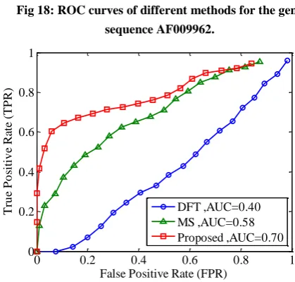
[image:7.595.22.562.453.690.2]

Finally, Figures 17-20 illustrate the ROC’s of the algorithms. It is obvious that the proposed algorithm has the highest value of its parameter over the other methods. By way of illustration, the area under the ROC curve is improved by the factor of 1.35, 1.74, 1.39 and 1.76 over the DFT and 1.9, 1.73, 1.57 and 1.2 over the MS filter in F56F11.4, AF009962, AF019074 and AJ223321 gene sequences, respectively. This implies that the proposed algorithm is superior to the other methods for identifying exonic gene regions.

Fig 9: Results of the (a) DFT, (b) MS-filter and (c) Proposed algorithms for identification of the exonic regions on the gene sequence F56F11.4.

(a)

(c)

(b)

0 1000 2000 3000 4000 5000 6000 7000 8000 9000 10000

0 0.2 0.4 0.6 0.8 1

Relative base location

Peri

o

d

-3

Po

w

er

Sp

ect

ru

m

0 1000 2000 3000 4000 5000 6000 7000 8000 9000 10000

0 0.2 0.4 0.6 0.8 1

Peri

o

d

-3

Po

w

er

Sp

ect

ru

u

m

(b)

(8)

0 1000 2000 3000 4000 5000 6000 7000 0

0.2 0.4 0.6 0.8 1

Peri

o

d

-3

Po

w

er

Sp

ect

ru

m

0 1000 2000 3000 4000 5000 6000 7000

0 0.2 0.4 0.6 0.8 1

Peri

o

d

-3

Po

w

er

Sp

ect

ru

m

0 1000 2000 3000 4000 5000 6000 7000

0 0.2 0.4 0.6 0.8 1

Peri

o

d

-3

p

o

w

er

Sp

ect

ru

m

0 1000 2000 3000 4000 5000 6000 7000 0

0.2 0.4 0.6 0.8 1

Peri

o

d

-3

Po

w

er

Sp

ect

ru

m

0 1000 2000 3000 4000 5000 6000 7000 0

0.2 0.4 0.6 0.8 1

Peri

o

d

-3

Po

w

er

Sp

ect

ru

m

0 1000 2000 3000 4000 5000 6000 7000

0 0.2 0.4 0.6 0.8 1

Peri

o

d

-3

Po

w

er

Sp

ect

ru

m

(a) (b)

(c)

(a) (b)

[image:8.595.47.590.78.353.2]

(c)

Fig 10: Results of the (a) DFT, (b) MS-filter and (c) Proposed algorithms for identification of the exonic regions on the gene sequence AF009962.

[image:8.595.56.581.414.672.2]

(9)

[image:9.595.47.585.83.339.2]

Fig 13. Comparison of sensitivity, specificity, and precision of the algorithms applied on F56F11.4 gene sequence by selecting different threshold levels. (a) Th=0.2, (b) Th=0.4, (c)

Th=0.6, and (d) Th=0.8.

0 500 1000 1500 2000 2500 3000 3500 4000 4500 5000 0

0.2 0.4 0.6 0.8 1

Relative base location,n

Peri

o

d

-3

p

o

w

er

s

p

ect

ru

m

0 500 1000 1500 2000 2500 3000 3500 4000 4500 5000

0 0.2 0.4 0.6 0.8 1

Peri

o

d

-3

Po

w

er

Sp

ect

ru

m

0 500 1000 1500 2000 2500 3000 3500 4000 4500 5000

0 0.2 0.4 0.6 0.8 1

Peri

o

d

-3

Po

w

er

Sp

ecrt

u

m

(a) _(b)

[image:9.595.52.583.431.674.2]

(c)

Fig 12: Results of the (a) DFT, (b) MS-filter and (c) Proposed algorithms for identification of the exonic regions on the gene sequence AJ223321.

Sensititvity Specificity Precision 0

0.2 0.4 0.6 0.8 1

DFT MS Proposed

(a)

Sensitivity Specifiicity Precision 0

0.2 0.4 0.6 0.8 1

DFT MS Proposed

(b)

Sensitivity Specificity Precision 0

0.2 0.4 0.6 0.8 1

DFT MS Proposed

(c)

0.2 0.4 0.6 0.8 1

DFT MS Proposed

(10)

[image:10.595.37.580.91.348.2]

Fig 15. Comparison of sensitivity, specificity, and precision of the algorithms applied on AF019074 gene sequence by selecting different threshold levels. (a) Th=0.2, (b) Th=0.4, (c)

[image:10.595.53.578.424.659.2]

Th=0.6, and (d) Th=0.8.

Fig 14. Comparison of sensitivity, specificity, and precision of the algorithms applied on AF009962 gene sequence by selecting different threshold levels. (a) Th=0.2, (b) Th=0.4, (c)

Th=0.6, and (d) Th=0.8.

0.2 0.4 0.6 0.8 1

DFT MS Proposed

(c)

0.2 0.4 0.6 0.8 1

DFT MS Proposed

(d)

0.1 0.2 0.3 0.4 0.5 0.6 0.7 0.8 0.9

DFT MS Proposed

(a)

0.1 0.2 0.3 0.4 0.5 0.6 0.7 0.8 0.9

DFT MS Proposed

(b)

0.2 0.4 0.6 0.8 1

DFT MS Proposed

(a)

0.2 0.4 0.6 0.8 1

DFT MS Proposed

(b)

0.2 0.4 0.6 0.8 1

DFT MS Proposed

(c)

0.2 0.4 0.6 0.8 1

DFT MS Proposed

(11)

P Sequence

F56F11.4

AF009962

Method

AF019074

AJ223321

0.2 0.4 0.6 0.8 1

DFT MS Proposed

0.2 0.4 0.6 0.8 1

[image:11.595.45.577.74.291.2]

DFT MS Proposed

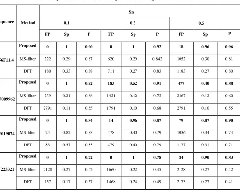
TABLE I. Quantitative evaluation of the algorithms result using Genbank datasets.

FP Sp P FP Sp P FP Sp

Proposed ₀ ₁ _0.90 ₀ ₁ _0.92 ₁₈ _0.96 _0.96

MS-filter 222 0.29 0.87 620 0.29 0.842 1052 0.30 0.81

DFT 180 0.33 0.88 711 0.27 0.83 1183 0.27 0.80

Proposed ₀ ₁ _0.92 ₁₈₃ _0.52 _0.91 ₄₇₇ _0.40 _0.88

MS-filter 239 0.21 0.88 1421 0.12 0.73 2467 0.12 0.60

DFT 2791 0.11 0.55 1791 0.10 0.68 2791 0.10 0.55

Proposed ₀ ₁ _0.84 ₁₄ _0.96 _0.87 ₇₉ _0.87 _0.90

MS-filter 24 0.82 0.83 478 0.40 0.79 1036 0.34 0.74

DFT 83 0.57 0.83 479 0.40 0.79 1177 0.31 0.71

Proposed ₀ ₁ _0.72 ₀ ₁ _0.78 ₈₄ _0.90 _0.83

MS-filter 2128 0.27 0.42 1660 0.22 0.45 2128 0.27 0.42

[image:11.595.65.562.359.755.2]

DFT 757 0.17 0.57 1468 0.24 0.49 2173 0.27 0.41

Fig 16. Comparison of sensitivity, specificity, and precision of the algorithms applied on AJ223321 gene sequence by selecting different threshold levels. (a) Th=0.2, (b) Th=0.4, (c)

Th=0.6, and (d) Th=0.8.

0.1 0.3 0.5

Sn

(c) (d)

0.1 0.2 0.3 0.4 0.5 0.6 0.7 0.8

DFT MS Proposed

(a)

0.2 0.4 0.6 0.8 1

DFT MS Proposed

(12)

[image:12.595.77.387.100.655.2] [image:12.595.93.533.105.427.2]

Fig 17: ROC curves of different methods for the gene sequence F56F11.4.

[image:12.595.326.536.143.423.2]

Fig 18: ROC curves of different methods for the gene sequence AF009962.

[image:12.595.73.292.433.642.2]

Fig 20: ROC curves of different methods for the gene sequence AJ223321.

TABLE II. Average computational time computed for the different algorithms.

Gene

identifier

Sequence

Length (bp)

Proposed algorithm

Multi-Stage filter DFT

F56F11.4 9833 11.93 714.97 718.40

AF009962 7422 14.62 712.24 391.06

AF019074 6350 12.04 710.17 282.04

AJ223321 5321 10.05 710.51 193.29

5. Conclusion

Gene identification is a complicated problem, and the detection of the period-3 patterns is a first step towards gene and exon prediction. Many different DSP techniques have been successfully applied for the identification task but still improvement in this direction is needed. In this paper, a fast

model-independent algorithm is presented for exon detection in DNA sequences. First, Z-curve representation was used to convert the symbolic sequence into digital signal. The Z-curve method decreases the computational cost by removing the one redundant sequence from the four binary indicator sequences in the Voss representation explained in [5] and [12]. Then, the

Average Computational Time (Second)

Fig 19: ROC curves of different methods for the gene sequence AF019074.

0 0.2 0.4 0.6 0.8 1

False Positive Rate (FPR)

T

ru

e

P

o

si

ti

v

e

Ra

te

(T

P

R)

DFT ,AUC=0.67 MS ,AUC=0.46 Proposed ,AUC=0.91

0 0.2 0.4 0.6 0.8 1

T

ru

e

P

o

si

ti

v

e

Ra

te

(T

P

R)

0 0.2 0.4 0.6 0.8 1

T

ru

e

P

o

si

ti

v

e

Ra

te

(T

P

R)

0 0.2 0.4 0.6 0.8 1

T

ru

e

P

o

si

ti

v

e

Ra

te

(T

P

R)

[image:12.595.333.543.440.640.2]

(13)

Linear Predictive Coding Model was used to reduce the correlation between the numerical data and therefore reduce the high frequency noise. Finally, the Goertzel algorithm was applied to the estimated sequence for the period-3 detection. The proposed algorithm minimizes the number of nucleotides incorrectly predicted as coding regions which leads to increase the specificity. Also, area under the ROC curve is improved in the proposed algorithm over the other tested methods. High speed characteristic is the major advantage of our algorithm which leads to decrease the run process of the algorithm.

6. REFERENCES

[1] Snustad D.P. and Simmons M.J., Principles of Genetics, John Wiley & Sons Inc., 2000.

[2] Dougherty E. R, et al., Genomic signal processing and statistics, EURASIP Book Series on Signal Processing and Communications, 2005.

[3] Fickett, J.W. and Tung CS, “Assessment of protein coding measures,” Nucleic Acids Res, PP. 6441-6450, 1992.

[4] Fickett, J.W, “The gene identification problem: an overview for developers,” Comput Chem, vol. 20, PP. 103-118, 1996.

[5] Vaidyanathan, P.P. and Yoon, B.J, “The role of signal-processing concepts in genomics and proteomics,” J. Franklin Inst, PP. 111-135, 2004.

[6] Tsonis, A. A., et al., “Periodicity in DNA coding sequences: implications in gene evolution,” J. Theor. Biol, vol. 151, pp. 323-351, 1991.

[7] Voss, R. F., “Evolution of long-range fractal correlations and 1/f noise in DNA base sequences,” Phy. Rev, Lett, vol. 85, pp. 1342-1345, 1992.

[8] Chatzidimitriou-Dreismann, C. A., and Larhammar, D., “Long-range correlations in DNA,” Nature, vol. 361, pp. 212-213, 1993.

[9] Henderson, J., et al., “Finding genes in DNA with a Hidden Markov Model,” J. Comput. Biol, vol. 4, pp. 127-141, 1997.

[10] Ding, C. H., and Dubchak, I., “Multi-class protein fold recognition using support vector machines and neural networks,” Bioinformatics, vol. 17, pp. 349-358, 2001.

[11] Eftestel, T., et al., “Eukaryotic gene prediction by spectral analysis and pattern recognition techniques,” In Proceedings of the Seventh IEEE Nordic Signal Processing Symposium, pp. 146-149, 2006.

[12] Anastassiou, D., “Genomic signal processing,” IEEE Sign. Proc. Mag, vol. 18, pp. 8-20, 2001.

[13] Fox, T. W., and Carreira, A., “A digital signal processing method for gene prediction with improved noise suppression,” EURASIP J. Appl. Aign. Proc, pp. 108-114, 2004.

[14] Tiwari S., Ramachandran S., Bhattacharya A., Bhattacharya S., and Ramaswamy R., “Prediction of probable genes by Fourier analysis of genomic sequences,” Comput Appl Biosci, vol. 13, pp. 263-270, 1997.

[15] Saberkari H., Shamsi M., Sedaaghi M. H., and Golabi F., “Prediction of protein coding regions in DNA sequences using signal processing methods,” 2012 IEEE Symposium

on Industrial Electronics and Applications (ISIEA 2012), Bandung, Indonesia, pp. 354-359, September 2012.

[16] Saberkari H., Shamsi M., and Sedaaghi M. H., “Identification of genomic islands in DNA sequences using a non-DSP technique based on the Z-Curve,” 11th Iranian Conference on Intelligent Systems (ICIS 2013),Tehran, Iran, 27-28 February 2013.

[17] Deng S., et al., “Prediction of Protein Coding Regions by Combining Fourier and Wavelet Transform”, Intarnational Conference on Image and Signal processing (ICISP), 2010. [18] Datta S., Asif A., “A Fast DFT-Based Gene Prediction

Algorithm for Identification of Protein Coding Regions,” Proceedings of the 30th International Conference on Acoustics, Speech, and Signal Processing, 2005.

[19] Akhtar M., Epps J., Ambikairajah E., “Signal Processing in sequence Analysis: advanced in Eukaryotic gene Prediction,” IEEE journal of selected topics in signal processing, 2008, vol. 2, pp. 310-321.

[20] Haykin S., Adaptive Filter Theory, Fourth Edition, Prentice Hall, 2001.

[21] Ma Baoshan., Zhu Yi-Sheng., “Kalman Filtering Approach for Human Gene Identification,” 2nd International Conference on Signal Processing Systems (ICSPS 2010), 2010.

[22] Ma Baoshan, “A novel adaptive filtering approach for genomic signal processing, “ IEEE 10th International Conference on Signal Processing (ICSP), 2010, pp. 1805-1808.

[23] Chakravarthy, N., et al., “Autoregressive modeling and feature analysis of DNA sequence,” EURASIP J. Appl. Sign. Proc, pp. 13-28, 2004.

[24] P. D. Cristea, “Conversion of nucleotides sequences into genomic signals,” J. Cell. Mol. Med., vol. 6, no. 2, pp. 279–303, 2002.

[25] P. D. Cristea, “Genetic signal representation and analysis,” In SPIE Conference, InternationalBiomedical Optics Symposium, Molecular Analysis and Informatics (BIOS ’02), vol. 4623 of Proceedings of SPIE, pp. 77–84, San Jose, Calif, USA, January 2002.

[26] J. M. Claverie, “Computational methods for the identification of genes in vertebrate genomic sequences,” Hum. Mol.Genet, vol. 6, no. 10, PP. 1735-1744, 1997. [27] W. F. Doolittle, “Phylogenetic classification and the

universal tree,” Science, vol. 284, no. 5423, pp.2124–2128, 1999.

[28] P. D. Cristea, “Genomic signals of chromosomes and of concatenated reoriented coding regions,” In SPIE Conference, Biomedical Optics (BIOS ’04), vol. 5322 of Proceedings of SPIE, pp. 29–41, SanJose, Calif, USA, January 2004, Progress in Biomedical Optics and Imaging, Vol. 5, No. 11.

[29] K.D. Rao and M.N.S. Swamy “Analysis of genomics and proteomics using DSP techniques,” IEEE Transactions on Circuits and Systems-1, vol. 55, no. 1, pp. 370-378, February 2008.

(14)

[31] Yan M., Lin Z. S., and Zhang C. T., “A new Fourier Transform approach for protein coding measure based on the format of the Z-curve,” Bioinformatics, vol. 14, no. 8, 1998.

[32] Rabiner L. R., Schafer R. W., Digital Processing of Speech Signals, Prentice-Hall, Inc, 1987.

[33]A.V. Oppenheim and R.W.Schafer, “Discrete Time Signal Processing,” Prentice Hall, Inc, NJ, 1999.

[34]Braun F. Q., “Nonrecursive digital filters for detecting multifrequency code dignals,” IEEE Transactions on Acoustic, Speech and Signal Processing, vol. ASSP-23, no. 3, pp. 250-256, 1975.

[35] Koval I., Gara G., “Digital MF receiver using discrete Fourier transform,” IEEE transactions on Commiunication, vol. COM-21, no. 12, pp. 1331-1335, 1973.

[36] Simington R. A. Z., and Percival T. M. P., “New frequency domain technique for DSP based VSAT modems,” Proc. IREE Conference, pp. 428-431, 1991.

[37] Burset M., and Guigo R., “Evaluation of gene structure prediction programs,” genomics, pp. 353-367, 1996.

[38] Fawcett T.,ROC Graphs: Notes and Practical Considerations for Researchers HP Laboratories, 2003.

[39] Ramachandran P., Lu W. S., and Antoniou A., “Optimized Numerical Mapping Scheme for Filter-Based Exon Location in DNA sing a Quasi-Newton Algorithm,” IEEE International Symposium on Circuits and Systems (ISCAS 2010), 2010.

[40] National Center for Biotechnology Information,National Institutes of Health,National Library of Medicine, http://www.ncbi.nlm.nih.gov/Genebank/index.html.