Automatic Detection of Retina Layers using Texture Analysis

Automatic Detection of Retina Layers using Texture

Analysis

Amineh. Naseri

Dept. of Computer & Information Technology,

Shahrood University of Technology Shahrood, Iran

Ali.Pouyan,

Dept. of Computer & Information Technology,

Shahrood University of Technology Shahrood, Iran

Nader.Kavian

Vitreoretinal Surgeon, Dr.khodadust Hospital

Shiraz, Iran

ABSTRACT

In this paper, two computer approaches is proposed for recognition of retina layers on optical coherence tomography (OCT) images. OCT uses the optical backscattering of light to scan the eye and describe a pixel representation of the anatomic layers within the retina. Our approaches is based on co-occurrence matrix for feature extraction and a neural network and a supervised learning method for classification, which four features of this matrix have been selected as a feature vector by support vector machine (SVM) and multilayer perceptron (MLP) have been used for classifying retina layers. Achieved results of combined these methods in the best state was 96.6% precision by MLP and 98.6% by SVM method. These results show that apply these methods on OCT images discriminate retina layers with efficient accuracy. Since, recognition of retina layers is important for automatic analyzing of OCT images, therefore our proposed methods can be very useful.

Keywords

Optical coherence tomography, Co-occurrence matrix, Multilayer perceptron, Support vector machine, Image segmentation

1.

INTRODUCTION

Optical coherence tomography is a powerful tool for ophthalmic imaging and can be used to visualize the retinal cell layers to detect and monitor a variety of retinal diseases. Cross-sectional images of retina are created by OCT. The retina layers will be visible as linear bright and dark bands using of A-scans in the OCT images. The retina layers with axial structures, like bipolar cells and photoreceptors, have lower backscatter than nerve fiber and plexiform layers which are in linear structures (Fig 1).

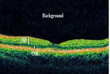
In these images, regular spatial repetition of gray level patterns is usually referred to as texture. Since, calculating the thickness of retina layers allows to determine the thickness of the whole retina that it will be very efficient for diagnosis of retina pathologies, in this work, two main retina layers (Fig2) are considered: the inner retina (IR), enclosing retinal nerve fiber layer, inner ganglion cells and inner plexiform layer, and the outer retina (OR), including outer plexiform and photo-receptor layers (thicker in fovea). In fact, they represent the most important features in clinical applications [1].

The OCT images are similar to ultrasound images and many their methods are based on these previous experiments. In a

multistep edge detection computer system, based on dynamic programming, and then they were described with texture analysis.

The nature of speckle noise [3] makes the application of 2D isotropic filters problematic. On the other hand, simple 1D edge detectors are not a useful method for detecting coherent retinal boundaries [4]. Different removing noise, edge-detection and filtering techniques were employed [5], [6]. Specifically, wavelet-based filtering that employs nonlinear thresholds [7], phase domain Processing approach [8], and anisotropic diffusion as improved in [9].

Fig 1: An OCT images with the labels for the retina layers

Also feature detection is known to be a necessary tool in image processing. Features such as edges have to be classified in a stable way to enable edge preserving image removing noise [10] and robust segmentation of image bounded by edges [11]. Moreover, region classification is very efficient for identifying the retina layers, because it is not sensitive to retina changes that occur in some retina disease.

For this reason, we decide analyze images in terms of texture features, is obviously region based. Therefore, a classical method has been selected for texture analysis. Descriptors of co-occurrence matrices of gray levels [12] have been then used for discriminating among two main retinal layers and the

Nerve fiber layer Ganglionp Cell layer

Inner plexiform layer

Inner nuclear layer

Outer plexiform layer Outer

nuclear layer External limiting membran e RPE

and choriocapillaris

Outer and inner photoreceptor

background. But other different approaches were proposed for describing texture [13].

In a same work [1], characteristics of co-occurrence matrices of gray levels have been used for discriminating among main retinal layers that for inner retinal layers, accuracy was 79% precision, slightly lower values were obtained for outer retinal layers.

Fig 2: A retinal OCT image with the labels indicating two main retinal layers

But in our work, have been used the co-occurrence matrix for demarcating two main layers of retina that obtained best accuracy has been achieved 96.6 % level of precision. This paper is structured as follows: Sections 2 and 3 contain a description of optical coherence tomography and texture analysis. Details of the approaches used for these images analysis are described in section 4. Section 5 includes the analysis of experiments and the results. Finally conclusions come in section 6.

2.

OCT SYSTEM

Optical coherence tomography (OCT) is an imaging modality analogous to ultrasound, but instead of using the difference in the flight times of acoustic waves (as in ultrasound), it uses light to achieve micrometer axial resolution. OCT is used in many different biomedical applications, with retinal imaging being the most successful and the driving force behind much OCT development. The axial resolution of OCT in retinal tissue is about 1-15 µm, which is 10 to 100 times better than ultrasound or MRI. Although relatively new to ophthalmology, a commercial OCT system has already revolutionized the field, rapidly becoming an essential tool in the diagnosis and monitoring of human retinal disease [14].

3.

TEXTURE

Texture is a result of local variations in brightness within one small region of an image. If the intensity values of an image are thought of as elevations, then texture is a measure of surface roughness [15].

A large body of literature exists for texture analysis of ultrasound, magnetic resonance imaging (MRI), computed tomography (CT), fluorescence microscopy, light microscopy, and other digital images.

In this work, have been used a study to determine how performance dependence matrices technique for using in classify OCT images of different tissues.

4.

METHODS

4.1

Feature Extraction

A set of texture features were extracted from the OCT tissue images. This set of features was the spatial gray-level dependency matrices (SGLDMs), or co-occurrence matrices [16].

A SGLDM is a spatial histogram of an image that quantifies the distribution of gray-scale values. SGLDMs were computed from the estimation of the second-order joint conditional probability density functions, sθ(i, j |d, θ). Each sθ (i, j |d, θ) was the probability of a pixel with a gray-level value (i) being (d) pixels away from a pix-el of gray-level value (j) in the (θ) direct-ion. If the image contained Ng gray levels, then an Ng × Ng matrix, sθ (i, j |d, θ), was created for each direction (θ) for a given distance (d) [17]. In this study, the direction took on one value, θ = 0◦, and distance was fixed at 1 pixel, so one SGLDMs were computed for each region. Four textural features were then used from each SGLDM including energy, correlation, homogeneity and inertia (also called contrast) for making feature vector. The SGLDM features for a particular angle are calculated as follows: Inertia: Returns a measure of the intensity contrast between a pixel and its neighbor over the whole image. The range of Inertia is between 0 and size (GLCM,1)-1) 2.

The formula is:



 

,

|

)



(

1

)

2 1

0 1

0

d

j

i

s

j

i

Intertia

L

i L

j













Correlation: Returns a measure of how correlated a pixel is to its neighbor over the whole image. The range of correlation is between -1 and 1. Correlation is 1 or -1 for a perfectly positively or negatively correlated image. Its formula is:













)

2

(

|

,

1

0 1

0

y x L

i L

j

i

j

s

i

j

d

n

correlatio









 

 









Energy: Returns the sum of squared elements in the GLCM. Range = [0 1]. The formula is:







,

|



(

3

)

2 1

0 1

0



 





i L

j

d

j

i

s

Energy









)

4

(

|

,

1

1

0 1

0

2

s

i

j

d

j

i

y

Homogeneit

L

i L

j





 









4.2

Classification

After feature extraction of images, a method has been used for classifying the pixels of images. Our proposed method is a neural network for classifying. This method employs four features of co-occurrence matrix as the feature vector.

4.2.1

Multilayer Perceptron

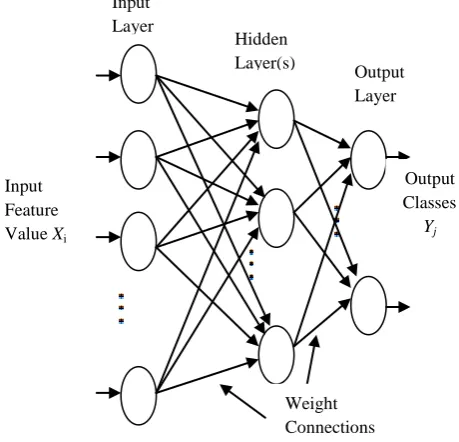
Multilayer perceptron (MLP) is a kind of supervised and most frequently neural networks. It consists of a network of nodes arranged in layers. A typical MLP network includes of various layers of processing nodes: an input layer that receives inputs, one or more hidden layers (depend on need of network), and an output layer which gets the classification results (Fig.3). Here, the main work is that when data are presented at the input layer, the network nodes perform calculations in the successive layers until an output value is obtained at each of the output nodes. This output should be able to indicate the appropriate class for the input data.

Fig 3: Architecture of a multilayer perceptron

A node in MLP can be modeled as an artificial neuron (Fig.4), which computes the weighted sum of the inputs and passes this sum through the activation function.

Fig 4: A node of MLP

Total process that has been done by a neuron is defined as follows:

Where W denotes the vector of wi that is the connection

weight between the input xi and the neuron, X is the vector of inputs xi, b is the bias and is the activation function, and Y is the output.

The MLP have been used in this study consists of three layers including an input layer, a hidden layer and an output layer that there are 4 neurons in input layer, 5 in hidden layer and 3 neurons in output layer. This network has been trained with five different learning rate and 500 iterations.

Here the MLP assigns a class membership to each pixel, based on its local texture features. For this reason, first OCT images are manually segmented by a technician. Our experiments have been done in two steps. In the first experiments ten images are used as a training set and other ten as a test set, and in the second experiments, training set contains fifteen images and other five images are used as test set. The results of second experiments are better than first experiments and best accuracy with this method is obtained 96% precision [18]. The results have been shown in Tables 1 and 2.

Table 1. Results of first step with MLP method

Classify Method

Multilayer percepteron

learning rate Accuracy

0.1 92.6667 %

0.2 92.6667 %

∑

x1

x2

x3

xm

.

.

.

w1

w2

w3

wm

b

+1

Y

Output Classes

Yj

Input Feature Value Xi

Weight Connections Input

Layer

Hidden

0.3 93.3333 %

0.4 93.6667 %

0.5 91%

Table 2. Results of second step with MLP method

Classify Method

Multilayer percepteron

learning rate Accuracy

0.1 96.6667 %

0.2 94.6667 %

0.3 91.3333 %

0.4 88.6667 %

0.5 88.6667 %

4.2.2

Support Vector Machine

Support vector machines (SVMs) are a set of related supervised learning methods used for classification and regression.

The utilization of support vector machine (SVM)[19], classifiers has gained high popularity in the last years. SVMs have achieved excellent recognition results in various pattern recognition applications [20]. Also it has been shown to be comparable or even superior to the standard techniques like Bayesian classifiers or multilayer perceptrons [21]. SVMs are discriminative classifiers based on Vapnik’s structural risk minimization principle.

Support Vector Machine (SVM) is primarily a classifier method that performs classification tasks by constructing hyper planes in a multidimensional space that separates cases of different class labels. SVM supports both regression and classification tasks. To construct an optimal hyper plane, SVM employees an iterative training algorithm, this is used to minimize an error function.

The SVM is only directly applicable for two-class tasks. But, we have to be applied algorithms that reduce the multi-class task to several binary problems.

Multiclass SVM aims to assign labels to instances by using support vector machines, where the labels are drawn from a finite set of several elements. The dominating approach for doing so is to reduce the single multiclass problem into multiple binary classification problems. Each of the problems yields a binary classifier, which is assumed to produce an output function that gives relatively large values for examples from the positive class and relatively small values for examples belonging to the negative class. Two common methods to build such binary classifiers are where each classifier distinguishes between (i) one of the labels to the rest versus-all) or (ii) between every pair of classes (one-versus-one). Classification of new instances for one-versus-all case is done by a winner-takes-all strategy, in which the

classifier with the highest output function assigns the class (it is important that the output functions be calibrated to produce comparable scores). For the one-versus-one approach, classification is done by a max-wins voting strategy, in which every classifier assigns the instance to one of the two classes, then the vote for the assigned class is increased by one vote, and finally the class with most votes determines the instance classification.

4.2.2.1

Kernel functions

There are a number of kernels that can be used in Support Vector Machines models. These include Linear, polynomial, radial basis function (RBF), PUK and sigmoid.

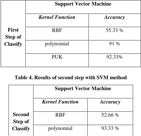
We apply SVM classifier for classifying two main layers of retina and background in OCT images. We used polynomial, RBF and PUK (Pearson VII Universal Kernel) kernels in SVM classify because best recognition level is achieved by these kernels, also evaluating the proposed method is achieved on two set of images. In this method, experiments have been done in two steps. In the first experiments ten images are used as a training set and other ten as a test set, and in the second experiments, training set contains fifteen images and other five images are used as test set)[22]. In Tables 3 and 4, the results of classify using the SVM is given. The results show which this method can be useful for retina layers classifying and best accuracy is achieved 98.6% precision with PUK kernel in second step of experiments (i.e. using fifteen images in train set and five images for test set.

Table 3. Results of first step with SVM method

First Step of Classify

Support Vector Machine

Kernel Function Accuracy

RBF 55.33 %

polynomial 91 %

PUK 92.33%

Table 4. Results of second step with SVM method

Second Step of Classify

Support Vector Machine

Kernel Function Accuracy

RBF 52.66 %

polynomial 93.33 %

PUK 98.66%

5.

EXPERIMENTAL RESULTS

In this paper, two automatic methods for recognition retina layers in OCT images are proposed.

vector machine for classifying. Four features of this matrix have been selected as a feature vector then are used by multilayer perceptron and support vector machine methods for classifying.

Achieved results of these methods for three main classes, background, IR and OR have been shown in Tables 1 to 4.These results show that above methods discern three main retina layers with efficient accuracy which achieved results of SVM method is better than MLP neural network. Moreover, we compared the recognition results of our methods and the images manually delineate by an expert. It was observed those four features of co-occurrence matrix and two methods for classifying has high accuracy and performance. Also calculating the thickness of IR and OR allows to determine the thickness of the whole retina that it will be very useful for diagnosis of retina pathologies.

6.

CONCLUSION

AND

FUTURE

WORKS

This study shows that texture analysis has the ability to provide a mean for diagnosing differentiation of tissue. Thus the presented method could have an important role in the future development of computer assisted OCT quantification techniques. For the example thickness and volume of the retina layers can help to diagnosis of damages. Moreover, the results show that it will be possible to segment the retina layers without the need of ultrahigh resolution systems. In the future work, our method will be extended to earlier detect pathology and can do the quantification of damage in eye pathologies by focusing only on the measurements from the retina layers that obtained in this work, also we will detect details of all retina layers exactly.

7.

REFERENCES

[1] M. Baroni, S. Diciotti, A. Evangelisti, P. Fortunato and A. La Torre3, Texture Classification of Retinal Layers in Optical Coherence Tomography, © Springer-Verlag Berlin Heidelberg (2007)

[2] Baroni M., Fortunato P., La Torre A. Towards quantitativeanalysis of retinal features in OCT. Med. Eng. & Phys. 29, 432-441, (2007)

[3] Schmitt JM, Xiang SH, Yung KM, Speckle in optical coherence Tomography. J. Biomed. Optics 4: 95-100, (1999)

[4] Ray R., Stinnett S.S., Jaffe G.J, Evaluation of Image Artefact Produced by Optical Coherence Tomography of Retinal Pathology. Am J Ophthalmol 139:18-29, (2005) [5] Koozekanani D., Boyer K., and Roberts C, Retinal

thickness measurements from optical coherence tomography using a Markov boundary model. IEEE Trans. Med. Imaging 20: 900–16, (2001)

[6] Shahidi M., Wang Z., Zelkha R, Quantitative Thickness Measurement of Retinal Layers Imaged by Optical Coherence Tomography. Am J Ophthalmol 139:1056– 61, (2005)

[7] S. H. Xiang, L. Zhou, and J. M. Schmitt, “Speckle noise reduction for optical coherence tomography, in Optical and Imaging Techniques for Biomonitoring III , H.-J.

Foth, R. Marchesini, and H. Podbielska, eds.”, Proc. SPIE 3196, 79, (1997).

[8] K. M. Yung, S. L. Lee, and J. M. Schmitt, “Phase-domain processing of optical coherence tomography images,” J. Biomed. Optics 4, 125 (1999)

[9] Cabrera Fernández D., Salinas H.M., Puliafito C.A, Automated detection of retinal layer structures on optical coherence tomography images. Opt. Express 13: 10200-216, (2005)

[10]D. Cabrera Fernández, and R. W. Knighton, “Active contour models for assessing lesion shape and area in OCT images of the retina,” Invest. Ophthalmol. Visual Sci. 44: E-Abstract 1770 (2003)

[11] J. Weickert, “Anisotropic diffusion filters for image processing based quality control,” A. Fasano, M. Primicerio eds., in Proc. Seventh European Conf. on Mathematics in Industry, (Teubner, Stuttgart, 1994),355-362

[12] Haralick R.M. Statistical and Structural Approaches to Texture. Proc.IEEE 67:786-804, (1979)

[13]T. Ojala, M. Pietikainen, and D. Harwood, A comparative study of texture measures with classification based on feature distributions. Pattern Recogn. 29: 51– 59, (1996)

[14]Accessed November 2009, from website http://www.Optical Coherence Tomography Vision Science and Advanced Retinal Imaging Laboratory [15]M.Oberholzer, M. Ostrecher, H. Christenm, and M.

Bruhlmann, Methods in quantitative image analysis, Histochem. Cell. Biol. 105, 333–355 (1996)

[16]F. Argenti, L. Alparone, and G. Benelli, Fast algorithms for texture analysis using co-occurrence matrices,IEEE Proc., Pt. F, 137(6), 443–448 (Dec. 1990).

[17]Kirk WGossage, Cynthia M Smith, Elizabeth M Kanter,Lida P Hariri, Alice L Stone, Jeffrey J Rodriguez ,Stuart K Williams1and Jennifer K Barton, Texture analysis of speckle in optical Coherence tomography images of tissue phantoms, (2006) .

[18]Amineh Naseri, Ali A. Pouyan, Nader. Kavian “An Image Processing Approach to Automatic Detection of Retina Layers Using Texture Analysis” Proceedings of the 17th Iranian Conference of Biomedical Engineering (ICBME2010(IEEE)), 3-4 November 2010.

[19]C. Burges. A tutorial on support vector machines for pattern recognition. Data Mining and Knowledge Discovery, 2(2):121–167,( 1998)

[20] N.Cristianini and J. Shawe-Taylor. Support Vector Machines. Cambridge University Press, (2000)