Solution of Linear Electrical Circuit Problem using Neural Networks

6

Solution of Linear Electrical Circuit Problem using Neural

Networks

J.Abdul Samath

Department of Computer Applications Sri Ramakrishna Institute of Technology, Coimbatore-641010,

Tamilnadu, India.

P.Senthil Kumar

Department of Computer Applications Sri Ramakrishna Institute of Technology, Coimbatore-641010,

Tamilnadu, India.

Ayisha Begum

Department of Information Technology VLB Janakiammal college of Engineering and Technology, Coimbatore-641008, Tamilnadu, India

ABSTRACT

In this paper, Neural network algorithm is introduced to study the singular system of a linear electrical circuit for time invariant and time varying cases. The discrete solutions obtained using neural network are compared with Runge-Kutta(RK) method and exact solutions of the electrical circuit problem and are found to be very accurate. Error graphs for inductor currents and capacitor voltages are presented in a graphical form to show the efficiency of neural network algorithm. This neural network algorithm can be easily implemented in a digital computer for any singular system of electrical circuits.

Keywords:

1.

INTRODUCTION

RK methods is used to determine numerical solutions of problems modeled as initial value problems involving differential equations that arise in the fields of science and engineering[1,10,11,12,20,25,26,27,28,29]. This method was derived by Runge around the year 1894 and extended by Kutta a few years later. They developed algorithms to solve differential equations efficiently and give solutions closer to the exact solutions.

Singular systems contain a mixture of algebraic and differential equations. In that sense, the algebraic equations represent the constraints to the solution of the differential part. These systems are also known as degenerate, descriptor or semi-state and generalized semi-state-space systems. The complex nature of singular system causes many difficulties in the analytical and numerical treatment of such systems, particularly when there is a need for their control. The system arises naturally as a linear approximation of system models or linear system models in many applications such as electrical networks, aircraft dynamics, neural delay systems, chemical, thermal and diffusion processes, large-scale systems, robotics, biology, etc.,[5,6,9,21]

Neural network or simply neural nets are computing systems, which can be trained to learn a complex relationship between two or many variables or data sets. Having the structures similar to

their biological counterparts, neural networks are representational and computational models processing information in a parallel distributed fashion composed of interconnecting simple processing nodes [33].

Neural networks could be used to provide a general link from measurements or device simulations to circuit simulation. The discrete set of outcomes of measurements or device simulations can be used as the target data set for a neural network. The neural network then tries to learn the desired behaviour. If this succeeds, the neural network can subsequently be used as a neural behavioural model in a circuit simulator after translating the neural network equations into an appropriate syntax-such as the syntax of the programming language in which the simulator is itself written. An efficient link, via neural network models, between device simulation and circuit simulation allows for the anticipation of consequences of technological choices to circuit performance. This may result in early shifts in device design, processing efforts and circuit design, as it can take place ahead of actual manufacturing capabilities: the device need not (yet) physically exist. Neural network models could then contribute to a reduction of the time-to-market of circuit designs using promising new semiconductor device technologies.

The mainstreams of electronic circuit theory and neural network theory will in forthcoming decades converge into general methodologies for the optimization of analogue nonlinear dynamic systems. As a demonstration of the viability of such a merger, a new modelling method will be described, which combines and extends ideas borrowed from methods and applications in electronic circuit and device modelling theory and numerical analysis [2,7,8,18,23,24] the popular error back propagation method (and other methods) for neural networks [3,4,13,14,22,31] and time domain extensions to neural networks in order to deal with dynamic systems [15,16,17,30,32].

2. STATEMENT OF THE PROBLEM

2.1 Study of Linear Electrical Circuit

7 Figure1. Electrical Circuit

This electrical circuit is governed by the following hybrid equations [34]

i1 0 0 -1 -1 v1 0 0

i4 = 0 0 0 1 v4 + 0 -1 Ea (1)

v2 1 0 0 0 i2 1 0 Jb

v3 -1 -1 0 1 i3 -1 0

Since ic = C c and v1 = Li1, substituting i1 = 2 1 , i2 = 2 2 ,

v3= 2i3 and v4 = 2i4 into (1) we then obtain

2 1 0 0 -1 -1 v1 0 0

.

i4 = 0 0 0 1 2i 4 + 0 -1 Ea (2)

v2 1 0 0 0 2 2 1 0 Jb

.

2 3 -1 -1 0 1 i3 -1 0

After re-arranging the terms, we obtain the singular system of equations as

K (t)=Ax(t)+Bu(t) (3)

With the initial condition x(0) = x0

where

2 2 0 0 0 0 -1 0 0 0 K = 2 2 0 0 A= -1 0 1 0 B= -1 0 0 0 0 0 1 -1 0 0 1 0 0 0 0 0 0 0 1 -1 0 -1

Where K is an n x n matrix, but singular in nature, therefore it is called singular systems. It is also called “generalized state space systems” or “descriptor systems”. A is an n x n matrix, B is an n x r matrix, x(t) is an n-state vector, and u(t) is an r-input vector.

In some cases, the variables have some inherent meaning such as voltage, current, position, velocity, or acceleration. or, the coefficient matrices have some special structures that may be lost by manipulating a system of the form in (3) into an ordinary state-space system.

By taking Ea = 1+ t + +

and Jb = 1 + t + t2 in (3) (4)

we obtain the exact solutions of (3) as

v1(t) = - - exp t

- + exp t

- 27t + – + 163

v2(t) = - - exp t

- + exp t (5)

- 26t +2t2 _{+ 164}

-14t + 2t2 _{+ 106}

i4(t) = - 93exp t – 93exp t

-15t + t2 _{+ 105}

v1(0) v2(0) i3(0) i4(0) T = 70 71 - 80 -81 T

The discrete solution of (3) with x(t) = [v1(t) v2(t) i3(t) i4(t)]T are

compared with the solutions obtained by Runge-Kutta method and Neural network method and are shown in tables 1 to 4 along with the exact solutions calculated using (5).

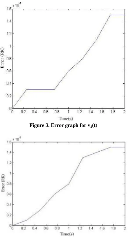
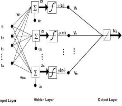
The errors in RK- method is represented by the graph for the variables v1(t), v2(t), i3(t) and i4(t) in Figures 2 to 5 at

8 i = fi (t, v) for i = 1, 2

i = fi (t, I) for i = 3, 4 (6)

In the following sections the above system will be solved by RK-method and Neural network approach respectively

.

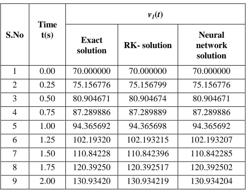
Table 1.Solutions of (3) and (5) for v1(t)

S.No

Time t(s)

v1(t)

Exact

solution RK- solution

Neural network solution

1 0.00 70.000000 70.000000 70.000000 2 0.25 75.156776 75.156799 75.156776 3 0.50 80.904671 80.904674 80.904671 4 0.75 87.289886 87.289889 87.289886 5 1.00 94.365692 94.365698 94.365692 6 1.25 102.19320

7

102.193215 102.193207 7 1.50 110.84228

5

110.842396 110.842285 8 1.75 120.39250

2

120.392517 120.392502 9 2.00 130.93420

4

130.934219 130.934204

Table 2.Solutions of (3) and (5) for v2(t)

S.No

Time t(s)

v2(t)

Exact

solution RK- solution

Neural network solution 1 0.00 71.000000 71.000000 71.000000 2 0.25 76.443237 76.443240 76.443237 3 0.50 82.571335 82.571338 82.571335 4 0.75 89.461761 89.461764 89.461761 5 1.00 97.199028 97.199034 97.199028 6 1.25 105.87549

6

105.875504 105.875496 7 1.50 115.59228

5

115.592296 115.592285 8 1.75 126.46021

3

126.460228 126.460213 9 2.00 138.60086

1

138.600876 138.600861

Table 3. Solutions of (3) and (5) for i3(t)

Table 4.Solutions of (3) and (5) for i4(t)

S. No

Time t(s)

i4(t)

Exact

solution RK-solution

Neural network solution

1 0.00 -81.000000 -81.000000 -81.000000 2 0.25 -91.060478 -91.060481 -91.060478 3 0.50 -102.182671 -102.182674 -102.182671 4 0.75 -114.473595 -114.473598 -114.473595 5 1.00 -128.052383 -128.052389 -128.052383 6 1.25 -143.051559 -143.051570 -143.051559 7 1.50 -159.618408 -159.618419 -159.618423 8 1.75 -177.916580 -177.916593 -177.916580 9 2.00 -198.127686 -198.127701 -198.127701

Figure 2. Error graph for v1(t)

S. No

Time t(s)

i3(t)

Exact

solution RK- solution

9 Figure 3. Error graph for v2(t)

Figure 4. Error graph for i3(t)

Figure 5. Error graph for i4(t)

3. RUNGE–KUTTA SOLUTION

RK algorithms have always been considered as the best tool for the numerical integration of ordinary differential equations (ODEs). Since system (6) contains n2 first order ODEs with n2 variables, RK method is explained for a system of two first order ODEs with two variables.

k11 (i + 1) = k11 (i) + (k1 + 2k2 + 2k3 + k4),

k12 (i + 1) = k12 (i) + (l1 + 2l2 + 2l3 + l4),

where

k1 = h * 11 (k11, k12),

l1 = h * 12 (k11, k12),

k2 = h * 11 (k11 + , k12 + ),

l2 = h * 12 (k11 + , k12 + ),

k3 = h * 11 (k11 + , k12 + ),

l3 = h * 12 (k11 + , k12 + ),

k4 = h * 11 (k11 + k3, k12 + l3),

l4 = h * 12 (k11 + k3, k12 + l3).

In the similar way, the original system(6) can be solved.

4. NEURAL NETWORK SOLUTION

In this approach, new feedforward neural network is used to change the trail solution of Eq. (6) to the neural network solution of (6). The trial solution is expressed as the difference of two terms as below (see [19]).

( i, j)a( t) = Aij – tNij (t, wij). (7)

The first term satisfies the TCs and contains no adjustable parameters. The second term employs a feedforward neural network and parameters wij correspond to the weights of the

neural architecture.

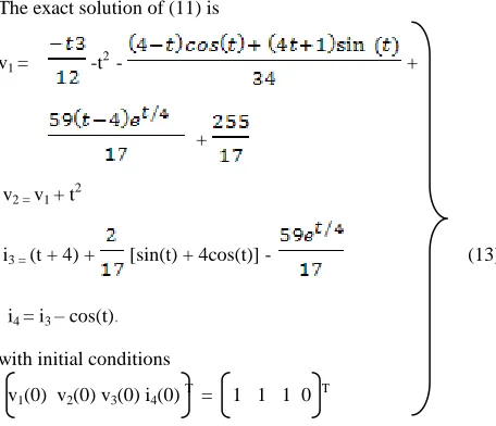
10 For a given input vector, the output of the network is

Nij = i) (zi) where zi = ij)tj + ui , wij denotes

the weight fromthe input unit j to the hidden unit i, vi denotes the

weight from the hidden unit i to the output, ui denotes the bias of

the hidden unit i and (z) is the sigmoidal transfer function.

The error quantity to be minimized is given by E = i, j)a - ij (t, ( i, j)a))

2

. (8)

The neural network is trained till the error function (8) becomes zero. Whenever E becomes zero, the trail solution (7) becomes the neural network solution of Eq.(6).

4.1 Structure of the FFNN

The architecture consists of n input units, one hidden layer with n sigmodial units and a linear output. Each neuron produces its output by computing the inner product of its input and its appropriate weight vector.

Fig. 6. Neural network architecture.

During the training, the weights and biases of the network are iteratively adjusted by Nguyen and Widrow rule [33]. The neural network architecture is given in the Fig. 6 for computing Nij. The neural network algorithm was implemented in

MATLAB on a PC, CPU 1.7 GHz for the neuro computing approach.

Neural network algorithm

Step 1. Feed the input vector tj.

Step 2. Initialize randomized weight matrix wij and bias ui.

Step 3. Compute zi = ijtj+ ui

Step 4. Pass zi into n sigmoidal functions.

Step 5. Initialize the weight vector vi from the hidden unit to

output unit.

Step 6. Calculate Nij = i (zi)

Step 7. Compute purelin function (Nij).

Step 8. Repeat the neural network training until the following error function

E = i, j)a - ij (t, ( i, j)a)) 2

= 0.

4.2 Study of Time-Varying Linear Electrical

Circuit

In this paper we applied Runge-kutta method for the time– invariant electrical circuit problem and the results are compared with Neural network algorithm for studying the time-varying electrical circuit, which is represented by a singular system.

Consider the electrical circuit depicted in Fig. 1 in section III. The following hybrid equation is obtained

.

2 2 0 0 1 0 0 -1 0 v1 0 0

0 0 2 2 2 = -1 0 1 0 v2 + -1 0 Ea

0 0 0 0 i3 1 -1 0 0 i3 1 0 Jb (10)

0 0 0 0 i4 0 0 1 -1 i4 0 -1

This is of the form

K (t) = Ax(t) + Bu(t) (11)

In order to study the effectiveness of the time varying singular system in electrical circuits, a hypothetical system is formed by transforming the matrices K, A, and B, which are basically time independent in (10) with time-varying components.

Hence, the singular system of the time-varying electrical circuit is of the form

2 2 0 0 1 0 0 -1 0 v1 0 0

0 0 2t 2t 2 = 0 0 t 0 v2 + -t 0 t

0 0 0 0 i3 1 -1 0 0 i3 t 0 cos(t)

0 0 0 0 i4 0 0 t -t i4 0 -t (12)

11 The exact solution of (11) is

v1 = -t 2

- +

+

v2 = v1 + t 2

i3 = (t + 4) + [sin(t) + 4cos(t)] - (13)

i4 = i3 – cos(t).

with initial conditions

v1(0) v2(0) v3(0) i4(0) T = 1 1 1 0 T

The discrete solutions of (12) have been determined using Neural network algorithm (with step-size h=0.25) in (3) and are compared with the exact solutions of (12) presented in (13) along with the solutions obtained by using the Runge-Kutta method. These results are presented in Tables 5 to 8. This Neural network algorithm yields more accurate results when compared to the Runge-Kutta method. Errors between the exact and discrete solutions are also given in Tables 5 to 8. To exhibit the efficiency of the discussed methods, an error graph is presented for the variables v1(t), v2(t), i3(t) and i4(t) in Figures. 7 to 10 at various time intervals. From this, we can observe that the Neural networks algorithm gives more accurate results when compared to the Runge-Kutta method.

Table 5.Solutions of (3) and (13) for v1(t)

S.No Time

t(s)

Time varying v1(t)

Exact solution

RK- solution Neural network solution

1 0.00 1.000000 1.000000 1.000000 2 0.25 0.960697 0.960700 0.960697 3 0.50 0.842521 0.842524 0.842521 4 0.75 0.646642 0.646646 0.646642 5 1.00 0.376276 0.376284 0.376276 6 1.25 0.036505 0.036516 0.036505 7 1.50 -0.366008 -0.366021 -0.366008 8 1.75 -0.823387 -0.823400 -0.823387 9 2.00 -1.326949 -1.326964 -1.326949

Table 6.Solutions of (3) and (13) for v2(t) S.No Time Time varying v2(t)

t(s) Exact

solution RK-solution

Neural network solution 1 0.00 1.000000 1.000000 1.000000 2 0.25 1.023197 1.023200 1.023197 3 0.50 1.092521 1.092524 1.092521 4 0.75 1.209142 1.209145 1.209142 5 1.00 1.376276 1.376280 1.376276 6 1.25 1.599005 1.599011 1.599005 7 1.50 1.883992 1.884000 1.883992 8 1.75 2.239113 2.239124 2.239113 9 2.00 2.673051 2.673066 2.673051

Table 7. Solutions of (3) and (13) for i3(t)

S. No Time

t(s)

Time varying i3(t)

Exact solution

RK-solution Neural network solution

1 0.00 1.000000 1.000000 1.000000 2 0.25 1.040643 1.040643 1.040643 3 0.50 1.036691 1.036694 1.036691 4 0.75 0.988188 0.988191 0.988188 5 1.00 0.896933 0.896936 0.896933 6 1.25 0.766301 0.766308 0.766301 7 1.50 0.600964 0.600975 0.600964 8 1.75 0.406530 0.406543 0.406530 9 2.00 0.189110 0.189125 0.189110

Table 8. Solutions of (3) and (13) for i4(t)

S.No

Time t(s)

Time varying i4(t)

Exact solution

RK-solution Neural network solution

12 Figure7. Error graph for v1(t)for time varying cases

Figure8. Error graph for v2(t)for time varying cases

Figure9. Error graph for i3(t)for time varying cases

Figure10. Error graph for i4(t)for time varying cases

5. CONCLUSION

The discrete solutions obtained using the Neural network algorithm gives more accurate values when compared to the RK-method. From tables 1 to 8, we observe that the solutions obtained by the Neural network match well with the exact solutions of the electrical circuit problem irrespective of whether they are time-invariant or time varying cases, but the RK- method yields a little error. From the error graphs presented in Figures 2 to 5 and 7 to 10, we can observe that the RK-method have errors in the solution.

6. REFERENCES

[1] R .K. Alexander and J.J. Coyle, “Runge-Kutta Methods for Differential-Algebric Systems,” SIAM J. of Numerical Analysis, vol. 27, no. 3, 1990, pp. 736-752.

[2] S.I.Amari “Mathematical Foundations of neurocomputing" Proc. IEEE, Vol. 78, pp. 1443-1463, Sep. 1990.

[3] J. A. Anderson and E. Rosenfeld, Eds., Neurocomputing: Foundations of Research.Cambridge, MA: MIT Press, 1988. [4] G.K.Boray and M.D.Srinath, ”Conjugate Gradient

Techniques for Adaptive Filtering," IEEE Trans. Circuits Syst.-I, Vol. 39, pp. 1-10, Jan. 1992.

[5] S.L.Campbell, Singular Systems of Differential Equations, Pitman, Marshfield, MA, 1980.

13 [7] L.O. Chua and P.M. Lin, Computer-Aided Analysis of

Electronic Circuits, Prentice-Hall, New Jersey, USA, 1975.

[8] L.O.Chua, C. A. Desoer and E. S. Kuh, Linear and Nonlinear Circuits. McGraw-Hill, 1987.

[9] L.Dai, Singular Control Systems, Lecture Notes in Control and Information Sciences, Springer Verlag, NewYork, 1989. [10] D.J. Evans, “A New 4th Order Runge-Kutta Method for

Initial Value Problems with Error Control,” Int.lJ. Computer Mathematics, vol. 139, 1991, pp. 217-227.

[11] D.J. Evans and A.R. Yaakub, “A New Fifth Order Weighted Runge-Kutta Formula,” Int.J.Computer Mathematics, vol. 59, 1996, pp. 227-243.

[12] D.J.Evans and A.R.Yaakub, “Weighted Fifth Order Runge-Kutta Formulas for Second Order Differential Equations,” Int. J.Computer Mathematics, vol. 70, 1998, pp. 233-239.

[13] P. Friedel and D.Zwierski, Introduction to Neural networks. (Introduction aux Reseaux de Neurones.) LEP Technical Report C 91 503, December 1991.

[14] D.Hammerstrom, “Neural networks at work," IEEE Spectrum, pp. 26-32, June 1993.

[15] R. Hecht-Nielsen, “Nearest matched filter classification of spatio- temporal patterns ", Applied Optics, Vol. 26,

pp. 1892-1899, May 1987.

[16] D. R. Hush and B. G. Horne, “Progress in Supervised Neural Networks," IEEE Sign.Proc. Mag., pp. 8-39, Jan. 1993.

[17] J. S. R. Jang, “Self-Learning Fuzzy Controllers Based on Temporal Back Propagation," IEEE Trans. Neural Networks, Vol. 3, pp. 714-723, Sep. 1992.

[18] D.R.Kincaid and E.W.Cheney, Numerical Analysis: Mathematics of Scientific Computing. Books/Cole Publishing Company, 1991.

[19] I.E. Lagaris, A. Likas, D.I.Fotiadis, Artificial neural networks for solving ordinary and partial differential equations, IEEE Trans.Neural Networks 9(1998) 987–1000. [20] J.D. Lambert, Numerical Methods for Ordinary Differential Systems. The Initial Value Problem, John Wiley & Sons,

Chichester, UK, 1991.

[21] F.L. Lewis, A Survey of linear singular systems, Circ. Syst. Signal Process. 5 (1986) 3–36.

[22] R.P. Lippmann, “An Introduction to Computing with neural Nets," IEEE ASSP Mag., pp. 4-22, Apr. 1987

[23] C. A. Mead, Analog VLSI and Neural Systems. Reading, MA: Addison-Wesley, 1989.

[24] P. B. L. Meijer, “Fast and Smooth Highly Nonlinear Table Models for Device Modeling," IEEE Trans. Circuits Syst., Vol. 37, pp. 335-346, Mar. 1990.

[25] K.Murugesan, D.Paul Dhayabaran, and D.J. Evans, “Analysis of Different Second Order Systems via Runge- Kutta Method,” Int. J.Computer Mathematics, vol. 70, 1999, pp. 477- 493.

[26] K.Murugesan, D.Paul Dhayabaran, and D.J. Evans, “Analysis of Different Second Order Multivariable Linear System Using Single Term Walsh Series Technique and Runge-Kutta Method,” Int. J. of Computer Mathematics, vol. 72, 1999, pp. 367-374.

[27] K. Murugesan, D. Paul Dhayabaran, and D.J. Evans, “Analysis of Non-Linear Singular System from Fluid Dynamics Using Extended Runge-Kutta Methods,” Int. Journal.Computer Mathematics, vol. 76, 2000, pp. 239- 266.

[28] K. Murugesan, D.Paul Dhayabaran, E.C. Henry Amirtharaj, and D.J. Evans, “A Comparison of Extended Runge-Kutta Formulae Based on Variety of Means to Solve System of IVPs,” International .Journal of Computer Mathematics, vol. 78, 2001, pp. 225-252.

[29] K. Murugesan, D. Paul Dhayabaran, E.C. Henry Amirtharaj and D.J. Evans, “A Fourth Order Embedded Runge-Kutta RKACeM(4,4) Method Based on Arithmetic and Centrodial Means with Error Control,” Int. J. Computer Mathematics, vol. 79, no. 2, 2002, pp. 247- 269.

[30] K. S. Narendra, K. Parthasarathy, “Gradient Methods for the Optimization of Dynamical Systems Containing Neural Networks," IEEE Trans. Neural Networks, Vol. 2, pp. 252- 262, Mar. 1991. 170 BIBLIOGRAPHY

[31] D.E . Rumelhart and J.L. McClelland, Eds., Parallel Distributed Processing, Explorations in the Microstructure of Cognition. Vols. 1 and 2. Cambridge, MA: MIT Press, 1986. [32] F. M. A. Salam, Y. Wang and M.-R. Choi, “On the analysis

of Dynamic Feedback Neural Nets," IEEE Trans. Circuits Syst., Vol. 38, pp. 196-201, Feb. 1991.

[33] Senjyu, T., Sakihara, H., Tamaki, Y., and Uezato, K. 2000. “Next Day Peak Load Forecasting using Neural Network with Adaptive Learning Algorithm Based on Similarity”. Electric Machines and Power Systems. 28(7):613- 624.