On the Performance of a Solar Driven Absorption Refrigerator

http://dx.doi.org/10.4236/epe.2014.69024

On the Performance of a Solar Driven

Absorption Refrigerator

Ali Fellah, Mouna Hamed, Ammar Ben Brahim

University of Gabes, Engineers National School, Applied Thermodynamic Research Unit, Gabes, Tunisia Email: [email protected]

Received 28 June 2014; revised 2 August 2014; accepted 15 August 2014

Copyright © 2014 by authors and Scientific Research Publishing Inc.

This work is licensed under the Creative Commons Attribution International License (CC BY). http://creativecommons.org/licenses/by/4.0/

Abstract

An endoreversible model is used to simulate the dynamic behavior of a solar driven absorption refrigerator, the cycle under different operating and design conditions. A global time minimization procedure is performed to reach maximum performances. To evaluate the influence of the cold temperature on the system’s performances, results are carried out for three values of this tem-perature. They are presented in normalized charts for general applications. The minimum time set point temperature, entropy and maximum refrigeration load are sharp and therefore, are im-portant to be considered for system design.

Keywords

Refrigeration, Solar Energy, Endoreversibility, Optimization, Transient Regime

1. Introduction

based on renewable sources of energy. Several authors presented studies of solar refrigeration systems in [3]-[6]. In the theory of classical thermodynamics, the cyclical model of an absorption refrigerator is treated in [7] as reversible four-heat-sources cycle, which consists of four reversible adiabatic and four reversible isothermal processes. In order to achieve the coefficient of performance (COP) of reversible four-heat-source refrigeration cycles, the isothermal parts of the cycle have to be carried out infinitely slow because of the presence of the thermal resistances. The cooling rate of the resulting refrigerates or trends to zero because an infinite time is taken to draw a finite amount of heat from the cooled space. Real absorption refrigerators are designed to deliver a certain amount of cooling load. It is usually too rough to predict the coefficient of performance of real absorp-tion refrigerators so that it is necessary to develop a new theory for absorpabsorp-tion refrigeraabsorp-tion cycles. Finite time thermodynamics (FTT) has emerged during the last three decades as a distinct subfield in heat transfer [8]. The method consists of the simultaneous application of heat transfer and thermodynamic principles in the pursuit of realistic models of heat transfer processes, devices, and installations, i.e., models that account for the inherent irreversibility of heat, mass, and fluid flow processes. The original objective of the finite time thermodynamics appears to reduce the differences between the predictions of classical thermodynamics and the results of real practice. The results obtained for varying thermodynamic cycle analyses by using FTT are closer to real device performance than those using classical thermodynamics [9]. In literature, several researches have been focusing on the performance optimization of refrigerators, based on endoreversible models in [10]-[12] and on irreversi-ble models in [13] [14].

Steady-state models are useful under several conditions, although under strongly dynamic conditions that are often seen in real-life operation, these models are unacceptably and inaccurate [15]. However, steady state mod-els do not provide time dependent information on the thermal behavior of absorption refrigerators and are there-fore not suitable for transient system simulations. In order to predict the performance of these chillers under all aspects of operation, dynamic simulations must be developed. Vargas et al. in [16] conducted a simulation of a solar collector driven water heating and absorption cooling plant using the three-heat-reservoir cycles via multi objective optimization. They concluded that the minimum pull-down and pull-up times, and maximum of the second law efficiencies found with respect to the optimized operating parameters are important. Recently, Hamed et al. in [17] presented a thermodynamic transient regime simulation of a solar driven absorption refri-gerator. An endoreversible model has been analyzed numerically to find the optimal conditions of a solar driven absorption refrigerator. Based on the latest reference, the main focus of this study is concentrated on the simula-tion of the transient behavior of the endoreversible model of a three heat reservoirs absorpsimula-tion heat transformer, with Newton’s heat transfer law with a detailed solar energy process. For a practical set of cold source tempera-tures 8˚C, 0˚C and −8˚C, the purpose of this paper is to investigate the effect of solar collector stagnation tem-perature and cold temtem-perature on time set point temtem-perature, entropy generated inside the cycle and finally eva-porator heat.

Solar collectors are broadly classified as, non-concentrating and concentrating type collectors. Flat-plate col-lectors are the most widely used kind of colcol-lectors in the world [18]. In this analysis, the collector adopted is a flat-plate collector. Flat-plate solar collectors are commonly used in solar space heating. It is economically adopted when the same collector is used for both heating and cooling spaces. However, regarding the relatively low temperatures attainable, only a few practical applications are available in flat-plate solar operated cooling processes.

2. Mathematical Model

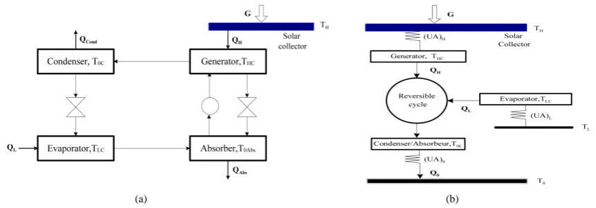
The solar driven absorption refrigeration cycle and its equivalent model are shown in Figure 1(a) and Figure 1(b). The cycle is considered to be endoreversible, i.e. internally reversible and externally irreversible. Internal irre-versibilities are assumed negligible in presence of the heat exchange irreirre-versibilities due to finite temperature differences. Internal irreversibilities due to heat transfer, throttling, mixing and internal dissipation of the work-ing fluid, which are responsible for the entropy generation are always present in a real heat driven refrigerator

[4].

Also, it is assumed that there is no heat loss between the solar collector and the generator and no work ex-change occurs between the refrigerator and its environment. The work input required by the solution pump is negligible regarding the energy input to the generator.

(a) (b)

Figure 1.(a) Schematic of a solar driven adsorption refrigeration system; (b) Equivalent endoreversible model.

ried out under a finite temperature difference and obey the linear heat-transfer law “Newton’s heat transfer law’’. Therefore, the steady-state heat transfer equations for the three heat exchangers can be expressed as:

(

) (

)

L L L LC

Q = T −T (1)

(

) (

)

H H H HC

Q = T −T (2)

(

) (

)

0 UA 0 0C 0

Q = T −T (3)

From the first law of thermodynamic:

0

H L

Q +Q =Q (4)

According to the second law of thermodynamic and the endoreversible property of the cycle, we have:

0

0

H L

HC LC C

Q

Q Q

T +T =T (5)

The generator heat input QH could be estimated by the following expression:

H sc sc

Q =η A G (6)

where Asc represents the collector area, G is the irradiance at the collector surface and ηsc stands for the

col-lector efficiency. The efficiency of a flat plate colcol-lector can be calculated, according to [3] and [5] as:

(

)

sc a b TH T

η = − − (7)

where a and b are two constants.

Equation (7) can be rewritten by introducing the collector stagnation temperature Tst as follows:

(

)

sc b Tst TH

η = − (8)

where Tst (for which ηsc =0) is given by:

0 st

T =T +a b (9)

The equation for heat input QH can be rewritten by combining Equations (6) and (8) as follows:

(

)

H sc st H

Q =A G b T −T (10)

The thermal inertia of the refrigerated space is large enough such that the transient operation of the refrigerator can be neglected when compared to the time evolution of the temperature inside the refrigerated space. The tran-sient regime of cooling is accounted for by writing the first law of thermodynamics, as follows:

(

) (

)

,air 0 load

d

UA d

L

v w L L

T

m c T T Q Q

t = − + − (11)

heat generated inside the refrigerated space. The factors

(

)

H,

(

)

(

)

The overall thermal conductance of the walls of the refrigerated space is given by

(

)

W. Since

(

)

(

)

L and

(

)

(

) (

) (

)

UA UA UA UA

H L

= + + (12)

According to the cycle model mentioned above, the rate of entropy generated by the cycle is described quanti-tatively by the second law as:

0 0 d d H L H L

Q Q Q

S

t = T −T −T (13)

To provide the model more general, a dimensionless form of the set of equations is preferred, using different reference parameters (as described below). Therefore, it is convenient to search for an alternative formulation that eliminates the physical dimensions of the problem. In a dimensionless model all variables are directly pro-portional to the dimensional ones presented in Equations (1) to (13).

The complete set of no dimensional equations for the model, including the absorption refrigerator steady state equations is:

(

)

L L LC

Q′ = Γ − Γz (14)

(

)

H H HC

Q′ = Γ − Γy (15)

(

)(

)

0 1 0C 1

Q′ = − −y z Γ − (16)

(

)

H st H

Q′ =B Γ − Γ (17)

H L

Q′ +Q′=Q′ (18)

0

0

H L

HC LC C

Q

Q′ Q′ ′

+ =

Γ Γ Γ (19)

(

)

d

1 d

L

L L

v Q Q

θ

Γ _{= − Γ + ′ − ′}

(20) 0 d d H L H L Q Q S Q θ ′ ′ ′ _′ = − −

Γ Γ (21)

where the following non-dimensional transformations are imposed:

0 0 0

0 0 0 0 0

0 0

0 0 0

load load 0 ,air , , , , , , , , ,

UA UA UA

UA

, , .

UA UA

H H L L st st

LC LC C C HC HC

H L

H L

sc

v

T T T T T T

T T T T T T

Q

Q Q

Q Q Q

T T T

Q A G b t

Q B

T θ m c

Γ = Γ = Γ =

Γ = Γ = Γ =

′ = ′ = ′=

′ = = =

(22)

here, B is the parameter which describes the size of the collector relative to the cumulative size of the heat ex-changers, and y, z and v are the conductance allocation ratios, defined by:

(

)

(

)

(

)

, ,

UA UA UA

w

H L

y= z= v= (23)

According to the constraint property of thermal conductance UA in Equation (12), the thermal conductance distribution ratio for the condenser can be written as,

(

)

UA

3. Simulation Results and Analysis

Using the models presented above, numerical simulations are conducted. The initial conditions are the heat gen-erated inside the refriggen-erated space

(

)

temper-ature in the refrigerated space. The system behavior is mainly determined by the driven hot tempertemper-ature and cooling temperature.

The principle main cooling applications are deep freezing (Γ = −_L 30 to −20˚C), ice making (Γ = −_L 5 to 0˚C) and chilling (Γ =_L 5 to 15˚C). The refrigerated space temperature to be achieved take three values 8˚C,

0˚C and −8˚C, in dimensionless parameters they are ΓL,set =0.943, ΓL,set =0.916 and ΓL,set =0.889. For

these three cases, the numerical results are shown in Figure 2 to Figure 8. The validated system model can be used to predict system performance at different operating states. The results of computations based on this anal-ysis are various and significant. They point out different operational regimes of the system, namely maximum power output or minimum dissipation (entropy generation) dependently on the studied case. Also, they show the limits of the variation range for the model variables, as well as reasons to choose the best solution between the physical ones.

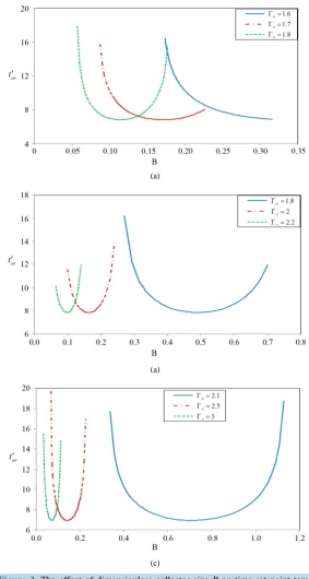
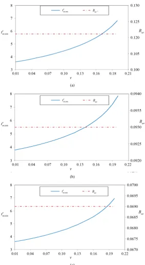
Time is an important factor in the cooling system for particular cooling period. Hence, at constant heat source temperature ΓH and for different values of the collector stagnation temperature Γst the variation of the time set

point temperature with the collector size is calculated (Figure 2).

The time set point temperature decreases gradually according to the collector size parameter until reaching a minimum time then it increases in each case of imposed collector stagnation temperature and refrigerated space temperature. The existence of an optimum for the thermal energy input QH′ is not due to the endoreversible

model aspects. However, an optimal thermal energy input QH′ results when the endoreversible equations are

constrained by the recognized total external conductance inventory, UA in Equation (12), which is finite, and the generator operating temperature TH. These constraints are the physical reasons for the existence of the

opti-mum point. The miniopti-mum time to achieve prescribed temperature is the same for different values of the stagna-tion temperature Γst. Then, for each imposed value of the stagnation temperature, the dimensionless collector

size parameter has a specific variation range decreasing continuously as the collector stagnation temperature in-creases. For example, at Γ =_L 0.889 and Γ =_st 2.1, B can vary between 0.337 and 1.126, while at Γ =_st 3, it varies from 0.034 to 0.111.

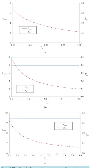
The results plotted in Figures 3-5 illustrate the minimum time θset,min to reach the desired set point

tempera-ture in the refrigerated space and the optimal parameter Bopt respectively against the stagnation temperature

st

Γ , thermal load inside the cold space Qload′ and conductance fraction v.

It can be observed from Figure 3 that the minimum time to achieve the prescribed temperature is independent of the collector stagnation temperature. This is due to the heat absorbed by the generator that is quite constant regarding the stagnation temperature variation [17]. If the generator heat input is constant, the dimensionless collector size B in Equation (17) will decrease with higher collector stagnation temperature and the temperature of the generator Equation (15) is also constant. The time set point temperature decreases with the increase of the refrigerated space temperature. For instance, at cold source temperature ΓL,set equal to 0.943, 0.916 and 0.889

the set point temperature θset values are respectively 6.83, 7.85 and 9.45.

This is due to the fact that the temperature of the evaporator starts to decrease linearly then it decreases. Here, the reaction of the evaporator is strongly affected by the generator behavior. Its temperature starts rising linearly, then it becomes stable. As the temperature of the generator is higher more heat is absorbed in the evaporator. While, the temperature of the evaporator decreases slowly, the temperature of the generator is maintained quit constantly, indicating that the equilibrium state has reached. As a result, the optimal dimensionless collector size B decreases monotonically as Γst increases. Also, one can see that the stagnation temperature Γst is limited,

its value of 1.8 for the first case

(

)

(

)

(

)

tem-perature ΓL,set desired which is not achieved.

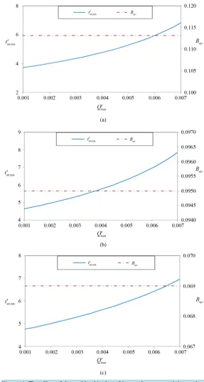
From the curves of Figure 4, as the stagnation temperature Γst and the heat source temperature ΓH are

constant, there is a clear proportionality between the minimum time set point temperature and the thermal load in the refrigerated space. The minimum time θset,min increases respectively when the thermal load Qload′

in-creases and the cold temperature ΓL decreases. This implies that the minimum time is strongly influenced by

(a)

(a)

(c)

Figure 2.The effect of dimensionless collector size B on time set point tem-perature. (a) Γ_L,set=0.943 , Γ =H 1.5; (b) ΓL set, =0.916 , Γ =H 1.5; (c)

,set 0.889 L

Γ = , Γ =H 1.5.

is absorbed at the evaporator, causing a decrease of the temperature of the evaporator. Also the cold temperature decreases with time. Figure 4 reveals that the thermal load inside the cold space has an almost negligible effect on optimal dimensionless collector size, whereas a decrease in the ΓL,set leads to a decrease in Bop.

(a)

(b)

(c)

Figure 3.The effect of collector stagnation temperature Γst on minimum time

set point temperature and optimal collector size. (a) Γ_L,set=0.943, Γ =H 1.5; (b) ΓL_,set=0.916, Γ =H 1.7; (c) ΓL,set=0.889, Γ =H 2.

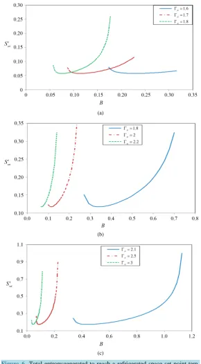
The total entropy generated inside the cycle function up to θset given in Equation (21) can be plotted with

re-spect to the dimensionless collector size B for various stagnation temperature parameters Γst and cold

tempera-ture and at constant heat source temperatempera-ture as shown in Figure 6.

(a)

(b)

(c)

Figure 4.The effect of thermal load in the refrigerated space on minimum time set point temperature and optimal collector size. (a) Γ_L,set=0.943, Γ =H 1.5,

1.5

st

Γ = ; (b) ΓL_,set=0.916, Γ =H 1.5, Γ =st 1.8; (c) ΓL,set=0.889, Γ =H

1.5 , Γ =st 2.

(a)

(b)

(c)

Figure 5.The effect of conductance fraction on minimum time set point tem-perature and optimal collector size. (a) Γ_L,set=0.943, Γ =H 1.5, Γ =st 1.8; (b)

,set 0.916 L

Γ = , Γ =H 1.5, Γ =st 1.8; (c) ΓL,set=0.889, Γ =H 2, Γ =st 3.

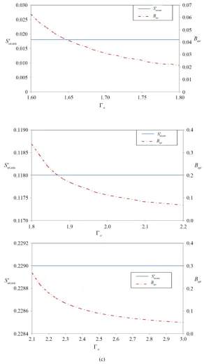
The optimization with respect to the stagnation temperature is pursued in Figure 7 for minimum total entropy generated up to set point temperature and optimal dimensionless collector size. It is observed that Sset,min′ is

in-dependent of Γst, whereas a decrease in the cold temperature leads to an increase in Sset,min′ . For instance, at a

cold source temperature ΓL,set equal to 0.943, 0.916 and 0.889 the minimum total entropy generated values are

(a)

(b)

(c)

Figure 6. Total entropygenerated to reach a refrigerated space set point tem-perature. (a) Γ_L,set=0.943, Γ =H 1.5; (b) ΓL,set=0.916, Γ =H 1.7 ; (c)

,set 0.889 L

Γ = , Γ =H 2.

is strongly affected by the time. It rises with the increase of time. On the basis of the second law of thermody-namics, the entropy production is always positive for an externally irreversible cycle.

From Figure 7, when the stagnation temperature increases then the collector optimal size decreases. This result brings to light the need for delivering towards the greatest values of Γst to approach the real refrigerator.

(c)

Figure 7. The effect ofdimensionless collector stagnation temperature on minimum entropy set point temperature and optimal collector size. (a) Γ_L,set=

0.943 , Γ =H 1.5; (b) ΓL,set=0.916, Γ =H 1.5; (c) ΓL,set=0.889, Γ =H 2.

(c)

Figure 8.The effect ofdimensionless collector size B on the heat absorbed by the evaporator. (a) ΓL,set=0.943, Γ =H 1.5; (b) ΓL set, =0.916, Γ =H 1.8; (c)

,set 0.889 L

Γ = , Γ =H 3.

regime when there is a refrigerant hot flow inside the evaporator that would heat the interior while the refrigera-tion system cooling capacity increases. When the steady state condirefrigera-tions are attained in the refrigerator the eva-porator heat transfer reaches a maximum. The maximum cooling capacity obtained for the tested refrigerator remains constant with the stagnation temperature. Then, for each imposed value of Γst, QL has a specific

varia-tion range continuously decreasing while B increases. The maximum evaporator heat transfer variavaria-tion shown by the curves increases when the cold temperature decreases, as is demonstrated with the result for

,set 0.943 L

It may be concluded that QL,max is more affected by ΓL,set than by Γst.

4. Conclusions

In this paper a dynamic model of a solar driven absorption refrigerator has been presented. An externally irre-versible but internally reirre-versible model has been employed to analyze the optimum conditions for which the maximum refrigeration effect can be achieved.

The cycle analysis has been studied under standard and variable working conditions. The results also supplied the initial conditions of the simulation of absorption performances. The existence of a collector optimal size for minimum time to reach a specified temperature in the refrigerated space, minimum entropy generation inside the cycle and maximum refrigeration rate was demonstrated. Appropriate dimensionless groups were identified and the generalized results reported in dimensionless charts.

The following conclusions could be derived:

• The minimum time to reach the prescribed temperature in the refrigerated space depends strongly on the cold temperature and the thermal load on the cold space but remains constant with the stagnation temperature variation.

• The minimum time set point temperature and collector optimal dimensionless size are influenced analogous-ly by the thermal load in the refrigerated space and by the thermal conductance of the walls.

• S_set,min′ is independent of Γst, whereas a decrease in ΓL,set leads to an increase in Sset,min′ .

• The maximum evaporator heat transfer increases when the cold temperature decreases, but remains constant as the stagnation temperature increases.

References

[1] Abdullah, M.O. and Hien, T.C. (2011) Comparative Analysis of Performance and Techno-Economics for a H2O-NH3- H2 Absorption Refrigerator Driven by Different Energy Sources. Applied Energy, 87, 1535-1545.

http://dx.doi.org/10.1016/j.apenergy.2009.10.018

[2] Calise, F., Denticed’Accadia, M. and Vanoli, L. (2011) Thermoeconomic Optimization of Solar Heating and Cooling Systems. Energy Conversion and Management, 52, 1562-1573. http://dx.doi.org/10.1016/j.enconman.2010.10.025

[3] Bejan, A. and Vargas, J.V.C. (1995) Optimal Allocation of a Heat Exchanger Inventory in Heat Driven Refrigerators. International Journal of Heat and Mass Transfer, 38, 2997-3004. http://dx.doi.org/10.1016/0017-9310(95)00045-B

[4] Chen, J. and Schouten, J.A. (1998) Optimum Performance Characteristics of an Irreversible Absorption Refrigeration System. Energy Conversion and Management, 39, 999-1007. http://dx.doi.org/10.1016/S0196-8904(97)10039-5 [5] Sokolov, M. and Hershgal, D. (1993) Solar-Powered Compression-Enhanced Ejector Air Conditioner. Solar Energy,

51, 183-194. http://dx.doi.org/10.1016/0038-092X(93)90095-6

[6] Vargas, J.V.C., Sokolov, M. and Bejan, A. (1996) Thermodynamic Optimization of Solar-Driven Refrigerators. Jour-nal of Solar Energy Engineering, 118, 130-135. http://dx.doi.org/10.1115/1.2847995

[7] Huang, F.F. (1976) Engineering Thermodynamics. Macmillan, New York.

[8] Bejan, A. (1995) Theory of Heat Transfer-Irreversible Power Plants-II. The Optimal Allocation of Heat Exchange Equipment. Journal of Heat and Mass Transfer, 38, 433-444. http://dx.doi.org/10.1016/0017-9310(94)00184-W

[9] Denton, J.C. (2002) Thermal Cycles in Classical Thermodynamics and Non Equilibrium Thermodynamics in Contrast with Finite Time Thermodynamics. Energy Conversion and Management, 43, 1583-1617.

http://dx.doi.org/10.1016/S0196-8904(02)00074-2

[10] Fellah, A., Khir, T. and Brahim, A.B. (2010) Hierarchical Decomposition and Optimization of Thermal Transformer Performances. Structural and Multidisciplinary Optimization, 42, 437-448.

http://dx.doi.org/10.1007/s00158-010-0505-y

[11] Bautista, O., Mendez, F. and Cervantes, J.G. (2003) An Endoreversible Three Heat Source Refrigerator with Finite Heat Capacities. Energy Conversion and Management, 44, 1433-1449.

http://dx.doi.org/10.1016/S0196-8904(02)00141-3

[12] Wijeysundera, N.E. (1999) Simplified Models for Solar-Powered Absorption Cooling Systems. Renewable Energy, 16, 679-684. http://dx.doi.org/10.1016/S0960-1481(98)00251-1

[13] Goktun, S. (1997) Optimal Performance of an Irreversible Refrigerator with Three Heat Sources. Energy, 22, 27-31.

http://dx.doi.org/10.1016/S0360-5442(96)00090-4

En-gineering, 16, 901-905. http://dx.doi.org/10.1016/1359-4311(95)00093-3

[15] Brown, M.W. and Bansal, P.K. (2002) Transient Simulation of Vapour-Compression Packaged Liquid Chillers. Inter-national Journal of Refrigeration, 25, 597-610. http://dx.doi.org/10.1016/S0140-7007(01)00060-3

[16] Vargas, J.V.C., Ordonez, J.C., Dilay, A. and Parise, J.A.R. (2009) Modeling, Simulation and Optimization of a Solar Collector Driven Water Heating and Absorption Cooling Plant. Solar Energy, 83, 1232-1244.

http://dx.doi.org/10.1016/j.solener.2009.02.004

[17] Hamed, M., Fellah, A. and Ben Brahim, A. (2012) Optimization of a Solar Driven Absorption Refrigerator in the Tran-sient Regime. Applied Energy, 92, 714-724.

[18] Chidambaram, L.A., Ramana, A.S., Kamaraj, G. and Velraj, R. (2011) Review of Solar Cooling Methods and Thermal Storage Options. Renewable and Sustainable Energy Reviews, 15, 3220-3228.