Adaptive Control Methodology for the Compensation of Linear and non Linear Parametric Disturbances

Adaptive control methodology for the compensation of

linear and non linear parametric disturbances

Karnakar Shukla

Dept. of computer science & engineering ,Institute of technology & management,Gida

Gorakhpur (UP)

Santosh Kumar Patel

Dept. of computer science & engineering ,Institute of technology & management,Gida

Gorakhpur (UP)

Vikas Kannaujia

Dept. of computer science & engineering ,Institute of technology

& management,Gida Gorakhpur (UP)

ABSTRACT

Adaptive controller is called for that provides a uniformly satisfactory performance in the presence of parametric uncertainties and variations. The adaptive approach to this problem is to design a controller with varying parameters, which are adjusted in such a way that they adapt to and accommodate the uncertainties and variations in the plant to be controlled by providing such a time-varying solution. The exact nature of which is determined by the nature and magnitude of the parametric uncertainties, the closed loop adaptive system seeks to enable a better performance. The result that have accrued in the field of adaptive control over the past three decades have provided a framework within which such time varying adaptive controller can be designed to yield stability and robustness in various control tasks. adaptive control deals with parametric uncertainties in control system and could be defined as the combination of a parametric estimator, which generate parameter estimates online with a control law in order to control class of plant (is the combination of process and actuator, which is a device that can influences the controlled variable of the process) whose parameter are completely unknown and/or could change with the time in a unpredictable manner. So from this paper we are trying to find auxiliary process variable that correlate well with the change in process dynamics. And also various approaches‟ to the manipulation with unpredictable parametric uncertainties

Keywords

parametric estimator, plant, actuator, control law,auxiliary process variable

1. INTRODUCTION:

We are going to represent a well known and interesting field of research in computer science since last few decades i.e. adaptive control ad by using this paper we focuses on a special topic adaptive control methodology for the compensation of linear and non linear parametric disturbances . our discussion start with the very brief introduction of adaptive control. The need of designing controller for dynamical system with the large parametric uncertainties was the initial motivation to introduce adaptive control. A major breakthrough in adaptive control occurred in 1980 when several research group [1]-[3] published result which showed that under certain ideal condition, it was possible to design globally stable adaptive systems.[4]and [5] show that in the presence of modeling error, such as bounded disturbances and/or unmodeled dynamics, an adaptive control scheme designed for stability in an ideal situation, could go

unstable. The main causes of instability were the adaptive cause of instability was the adaptive law for estimating the unknown parameters that made the closed-loop system nonlinear and more susceptible to the effects of modeling errors. Adaptive control has a long and vigorous history” since As introduced by [6] “Research in adaptive the initial study in 1950s on adaptive control which was motivated by the problem of designing autopilots for air-craft operating at a wide range of speeds and altitudes. With decades of efforts, adaptive control has become a rigorous and mature discipline which mainly focuses on dealing parametric uncertainties in control systems, especially linear parametric systems. and also it is stated in [7] i.e. From the initial stage of adaptive control, this area has been aiming at study how to deal with large uncertainties in control systems. This goal of adaptive control essentially means that one adaptive control law cannot be a fixed controller with fixed structure and fixed parameters because any fixed controller usually can only deal with small uncertainties in control systems. The fact that most fixed controllers with certain structure (e.g. linear feedback control) designed for an exact system model (called nominal model) can also work for a small range of changes in the system parameter is often referred to as robustness, which is the kernel concept of another area, robust control.

2.APPROACHES

TO

ADAPTIVE

CONTROL:

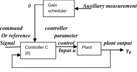
2.1 Gain Scheduling:

using some suitable design approach. The controller is tuned for each operating condition. The stability and performance of the system are evaluated at different operating condition. It turns out that in the case of scheduling on an exogenous parameter, this amounts to requiring the parameter to vary sufficiently slowly. In the case of a nonlinear plant scheduling on a plant output, this amounts to requiring the plant output to vary sufficiently slowly and capture the plant nonlinearities. Note that these are precisely the intuitive ideas which have guided existing gain-scheduled designs.

𝜃 Auxiliary measurement

command controller

Or reference parameter Signal control plant output

Input u 𝐲𝐩

Figure 1: gain scheduling controller

According to [8] since gain scheduled designs are based on

linearization, the limitation of capturing the non linear ties can be addressed in the appropriate selection of the scheduling variables. In this case , any theory developed is likely to simply verify the intuition obtained from an understanding of the physical system. The case of the restriction to slow variation on the scheduling variable most likely is due to the nature of the scheduling algorithms. More precisely , the scheduling of controller gains is such that good performance may be expected for any fixed interpolated operating condition. However, performance may deteriorate rapidly as one experiences rapid changes throughout the range of operating conditions(as an example ,such rapid changes may be expected in missile trajectories[9]). The advantage of gain scheduling is that the parameter can be changed quickly in response to change in the plant dynamics depend in the plant dynamics. It is convenient especially if the plant dynamics depend in a well-known fashion on a relatively few easily measurable pressure-that is the product of the air density and the relatively velocity of the aircraft squared. The disadvantage of gain scheduling is that it is open loop adaptation scheme, with no real learning or intelligence. [6]

2.2 Model Reference Adaptive Control:

The idea behind MRAS is to create a closed loop controller, in which parameters are updated as per the response of the system. The output is compared with the desired response from a reference model. The controller parameters are updated based on this error..

𝑦𝑚

r - 𝑒0

∑ +

U y

[image:2.595.303.532.86.210.2]

Figure 2: model reference adaptive control

A good understanding of the plant and the performance requirements it has to meet allow that the designer to come up with a model referred to as the reference model, that describe the desired i/o properties of the closed –loop plant. The objective of MRAC is to find the feedback control law that changes the structure and dynamics of the plant so that its I/O properties are exactly the same as those of the reference model.The reference model is designed so that for a given reference input signal

𝑟 𝑡 the output 𝑦𝑚 𝑡 of the reference model represents the

desired response the plant output y(t) should follow. The feedback controller denoted by C 𝜃𝑐∗ is designed so that all signals are bounded and the closed-loop plant transfer function from r to y is equal to 𝑊𝑚 𝑠 . This transfer function matching

guarantees that for any given reference input 𝑟 𝑡 , the tracking error 𝑒1≅ 𝑦 − 𝑦𝑚, which represents the deviation of the plant output from the desired trajectory 𝑦𝑚, converges to zero with

time. The transfer function matching is achieved by canceling the zeros of the plant transfer function G(s) and replacing them with those of 𝑊𝑚 𝑠 through the use of the feedback controller

C 𝜃𝑐∗ The cancellation of the plant zeros puts a restriction on

the plant to be minimum phase, i.e., have stable zeros. If any plant zero is unstable, its cancellation may easily lead to unbounded signals.[10]

The design of C 𝜃𝑐∗ requires the knowledge of the coefficients of the plant transfer function G(s). If 𝜃∗ is a vector containing all the coefficients of

G(s) = G(𝑠, 𝜃∗), then the parameter vector C 𝜃𝑐∗ may be computed by solving an algebraic equation of the form

𝜃𝑐∗=𝐹 𝜃∗

When 𝜃∗ is unknown the MRC scheme of Figure 1.8 cannot be

implemented because 𝜃𝑐∗cannot be calculated using (1.2.3) and

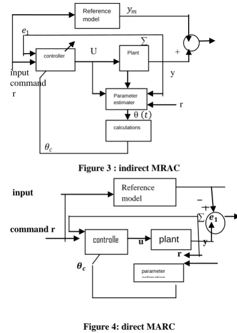
is, therefore, unknown. One way of dealing with the unknown parameter case is to use the certainty equivalence approach to replace the unknown 𝜃𝑐∗ in the control law with its estimates 𝜃𝑐 𝑡 obtained using the direct or the indirect approach. The resulting control schemes are known as MRAC and can be classified as indirect MRAC shown in Figure 1.9 and direct MRAC shown in Figure 1.10.

Gain scheduler

Controller C (θ)

Plant

Controller _Plant

[image:2.595.54.275.211.327.2]

𝑦𝑚

- 𝑒1

∑ U +

input y command

r r θ 𝑡

[image:3.595.44.277.69.395.2]

𝜃𝑐

Figure 3 : indirect MRAC

input

∑ 𝒆𝟏

command r

u y r 𝜽𝒄

Figure 4: direct MARC

2.3 Self Tuning Regulators:

Self tuning regulator form an important sub-class of adaptive control. The self tuning regulator (STR )attempts to automate several tasks such as modeling , design of a control law, implementation and validation.th given figure illustrated which shows the block diagram of a process with an STR. it is assumed that the structure of the process is specified. Parameters of the process are estimated on-line by the block labeled „parameter identifier‟. The block labeled controller tuner‟ contains computations that are required to perform the design of a controller with a specified method and a few design parameters that can be chosen externally. The design problem is called the underlying design problem for systems with known parameters. The block labeled „controller‟ is an implementation of the controller whose parameters are obtained from the „controller tuner‟ block [6] The design of an STR can be divided into sub-tasks such as designing the modules for parameter estimation [] and controller design []..The design method is summarized by a controller structure, and a relationship between plant parameters and controller parameters. Since the plant parameters are in fact unknown, they are obtained using a recursive parameter identification algorithm. The controller parameters are then obtained from the estimates of the plant parameters, in the same way as if they were the true parameters. This is usually called a certainty equivalence principle. The resulting scheme is represented on figure 0.4 the self tuning approach was originally proposed by Kalman[1958] and clarified by Astrom & Wittenmark[1973].The self tuning regulator is very flexible with respect to its choice of controller design methodology (linear quadratic, minimum variance, gain-phase margin design..), and the choice of identification scheme(least square; maximum like hood, extended Kalman filtering….) .The analysis of self tuning adaptive system is however more complex than the analysis of model reference scheme, due primarily to the(usually nonlinear)

transformation from identifier parameters to controller parameters.[1]

SPECIFICATION PROCESS

PARAMETER U

CONTROLLER &PARAMETERS

REFERNCE + ∑ OUTPUT

\ _ CONTROL SIGNAL

[image:3.595.294.542.108.324.2]

figure 5: self tuning controller

2.4 Direct and Indirect Adaptive Control:

These two different approaches of adaptive control different and both refers two different approaches of adaptive control methodology direct basically referrers to model reference adaptive control and indirect referrers to self tuning regulator .The self tuning regulator first identifies the plant parameter recursively, and then uses these estimates to update the controller parameters through some fixed transformation. The model reference adaptive schemes update the control loop parameter directly .the model reference adaptive schemes can be seen as a special case of the self tuning regulators, with an identity transformation between updated parameter and controller parameters.

2.5 Stochastic Control Approach:

Adaptive controller structure based on model reference or self tuning approach is based on heuristic arguments. Yet it would be appealing to obtain such structure from a unified theoretical framework. This can be done (in principle, at least) using stochastic control. The system and its environment are described by a stochastic model, and a criterion is formulated to minimize the expected value of a loss function, which is a scalar function of state and controls. It is usually very difficult to solve stochastic optimal control problems (a notable exception to solve stochastic optimal control problems).when indeed they can be solved, the optimal controller have the structure shown in figure 0.5; an identifier (estimator) followed by a non linear feedback regulator.

Reference model

controller Plant

Parameter estimater

calculations

controlle r

plant

parameter estimation

CONTROLLER TUNNER

Parameter identifier

Dynamic process

CONTROLLER

Reference Signal r control Single u plant

output

YP

Figure 6: “generic” stochastic controller

The estimator generates the conditional probability distribution of the state from the measurement, this distribution is called the Hyperstate (usually belonging to as an infinite dimensional vector space).the self tuner may be thought of as an approximation of this controller, with the Hyperstate approximated by the process state and process parameters estimate. [9]

3. A SIMPLE EXAMPLE:

Because of the nonlinearity and time varying system Adaptive control system are always being difficult to analyze and also difficult when the plant they are controlling are linear, and time invariant. This leads to interesting and delicate technical problems with a simple example. We also discuss some of the adaptive schemes of the previous section in this context. We consider a first order, time variant, linear system with transfer function

𝑃 (s) = _𝑠+𝑎kp (1)

Where a>0 is known. The gain 𝐾𝑃 of the plant is unknown, but

its sign is known (say 𝐾𝑃>0).The control objective is to get plant

output to match a model output, where the reference model transfer function is

𝑀(s)=_𝑠+𝑎1 (2)

Only gain compensations –or feed forward control –is

[image:4.595.52.290.87.198.2]

necessary, namely a gain θ at the plant input, as is shown on figure 0.6. [1]

𝑀

𝒚𝒎

r - 𝒆𝟎 𝑷 +

+ 𝛉 𝒚𝒑

Figure 7: simple feed forward controller

Note that if 𝐾𝑃 were known, θ would logically be chosen to be 1

/ 𝐾𝑃. We will call-

θ*= 1 / 𝐾𝑃 (3)

The nominal value of the parameter θ that is the value which realizes the output matching objective for all inputs. The design

3.1 Gain Scheduling:

Let v (t) ∈ IR be some auxiliary measurement that correlate in known fashion with𝐾𝑃, say 𝐾𝑃(t) = 𝑓 𝑣(𝑡) . Then the gain

scheduler choose at time t

θ (t)= _{𝑓 𝑣(𝑡)} 1 (4)

3.2 Model Reference Adaptive Control Using

the M.I.T Rule:

To apply the M.I.T rule, we need to obtain 𝜕e0 (θ) / 𝜕θ = 𝜕 yp (θ) / 𝜕θ, with the understanding that θ is frozen. From figure 0.6, it is easy to see that

𝜕𝑦_𝜕𝜃𝑝(θ) = _𝑠+𝑎𝐾𝑝 =𝑘𝑝𝑦𝑚 (5) we see immediately that the sensitivity function in above

equation depends on the parameter𝑘𝑝 which is unknown, so that 𝜕yp/ 𝜕θ is not available. However the sign of 𝑘𝑝 is known (𝑘𝑝>0), so that we may merge the constant 𝑘𝑝 with the

adaptation gain. The M.I.T rule becomes 𝜃 = -g e0 𝑦𝑚 g>0 (6)

Note that above equation prescribes an update of the parameter θ and the model output 𝑦𝑚 . [4] [10]

3.2.2 Model Reference Adaptive Control

Using the

Lyapunov Redesign:

The control schemes are exactly as before, but the parameter update law is chosen system .the plant and reference model are described by…

𝑦 p= - a 𝑦𝑝 + 𝑘𝑝θr (7)

𝑦 m = - a 𝑦𝑚 + r = -a𝑦𝑚 +𝑘𝑝θ*r (8)

Subtracting (8) from (7) we get, with e0= 𝑦𝑝 - 𝑦𝑚

𝑒 0 = -a e0+ 𝑘𝑝 (θ -θ*) r (9) Since we would like θ to converge to the nominal value θ

*=1/𝑘𝑝, we define the parameter error as

∅ = θ – θ* (10) Note that since θ * is fixed (though unknown), ∅ = θ .

The Lyapunov redesign approach consist in finding an update law so that the Lyapunov function

V (e0, ∅)=e0 2

+kp∅ 2

(11) Is decreasing along trajectories of the error system

𝑒0 = - a e0+kp∅r

∅ = update law to be defined (12) Note that since 𝑘𝑝 >0, the function v (e0,∅) is a positive definite

function. The derivative of v along the trajectories of the error system (12) is given by

𝑣 (e0, ∅)(12) = - 2 a e02+2kp e0 ∅r + 2kp∅∅ (13) Choosing the update law

𝜃 = ∅ = -e0r (14) Yields

𝑣 (e0, ∅) = -2a e02 ≤ 0 (15) Thereby guaranteeing that e02+kp∅2 is decreasing along the

trajectories of (12), (14) that e0, and ∅ are bounded. Since v (e0,

∅) is decreasing and bounded below, it would appear that e0→0

as t→∞. This actually follows from future analysis, provided that r is bounded (cf. Barabalat‟s lemma 1.2.1). [4][10]

CONTROLLER

PLANT

HYPERSTATE CALCULATION

𝐼

𝑆+𝑎 Type equation here.

a

𝐾𝑃

[image:4.595.55.239.575.693.2]

4. CONCLUSION

Using this paper we have tried to figure out all the preexisting different approaches to cooperate well with the parametric uncertainties in both linear and non-linear adaptive system we have mainly focused on gain scheduling, MARC, self tuning and stochastic adaptive control that effectively for handling these parametric uncertainties. We have pointed out all those approaches that are initially introduced, by taking the some the references as well as recent used approaches. And also using an simple example we tried to show that even when simple feed forward control of a linear, time invariant, first order plant was involved, the analysis of the resulting closed-loop dynamics could be involved: the equations were time-varying equation once feedback control is involved, the equation becomes non linear and time varying. Overall summary of this paper to pointed out all the those approaches which are proposed are being applied for the compensation of parametric disturbances.

5

.

REFERENCES

[1] A. S. Morse, “Global stability of parameter adaptive control systems, ”IEEE Trans. Automat. Contr., vol. AC-25, pp. 433439, June 1980.

[2] K. S. Narendra, Y. H. Lin, and L. S. Valavani, “Stable adaptive controller design-Part It Proof of stability,” IEEE Trans. utomat. Contr., vol.

[3] G. C. Goodwin, P. J. Ramadge, and P. E. Caines, “Discrete

time AC-25, pp. 440-448, June 1980. multivariable adaptive control,” IEEE Trans. Automat. Conrr., vol. AC-25, pp. 449-456. June 1980.

[4] P. A. Ioannou and P. V. Kokotovic, Aduptive Systems with

Reduced Models, Berlin. Springer-Verlag, 1983.

[5] C. E. R o b , L. Valavani, M. Athans, and G. Stein,

“Robustness of continnous-time adaptive control

algorithms in the presence of unmodelled dynamics,” IEEE

Trans. Automat. Conrr., vol. AC-30, no.9, pp. 881-889, Sep. 1985.

[6] Adaptive control: stability, convergence and robustness by

Shanker Shastry and Marc Bodson, pp .2-16, 1994

[7] Adaptive Control, Edited by Kwanho You p. cm. ISBN

978-953-7619-47-31. Adaptive Control I. Kwanho You

[8] Gain scheduling: potential hazards and possible remedies By jeff s.shamma and mical athans Ieee control system

[9] R.Reichert, “Mordel robust control for missile autopilot design,” in proc.1990 acc,san dieago, ca

[10]Loapunov, P. A., “Robust Adaptive Controller with zero Residual tracking Error,” IEEE Trans .On Automatic, vol. AC-31, no. 8, pp. 773-776, 1986.

[11]Stochastic Control,” IEEE Trans On Automata Control,

Vol. AC - 19, no. pp 494-500, 1974.

[12]Sastry, S., “Model-Reference adaptive control- Stability, Parameter convergence, and Robustness”, I.MA Journal of Mathematical control & information, Vol. 1, pp. 27-66, 1984.

[13]Dugard, L., & J.M. Dion, “Direct Adaptive Control for Linear System”, int. J. Control, Vol. 42, no. 6, pp. 1251-1281, 1985.

[14]Design of a Fractional-order Self-tuning Regulator using Optimization Algorithms Deepyaman Maiti, Mithun Chakraborty, Ayan Acharya, and Amit Konar Department of Electronics and Telecommunication Engineering, Jadavpur University, Kolkata, India Proceedings of 11th International Conference on Computer and Information Technology (ICCIT 2008)25-27 December, 2008, Khulna, Bangladesh. 1-4244-2136-7/08/$20.00 ©2008 IEEE.

[15]Landau, Y.D., Adaptive control- The Model Reference