http://dx.doi.org/10.4236/jss.2015.33010
Dynamic Pricing of Perishable Products with
Competition
Weiwei Ji
School of Economics and Management, Nanjing University of Science and Technology, Nanjing, China Email: [email protected]
Received February 2015
Abstract
With the development of product development technology and the rapid rise of online retailing, the market competition becomes increasingly fierce. Based on consumer utility function, this ar-ticle established a two-stage dynamic pricing model and discussed pricing strategies under con-sumer behavior and market competition. Findings indicate that product quality difference and consumer valuation decreasing coefficient determine the order of the consumer purchase deci-sions. The firm who provides lower-quality products suffered more loss than the firm who pro-vides high-quality products.
Keywords
Dynamic Pricing; Perishable Products; Competition
1. Introduction
With the development of Internet, competition between firms becomes increasingly fierce. Besides, replacement of product is becoming faster and faster, consumers also are becoming more and more “smart”. These all in-crease competition among firms. In the competitive environment, firms not only consider consumers’ behavior, but also consider the impact of competitors’ pricing strategies.
Literature related to this paper is dynamic pricing with competition in revenue management. Based on dis-counted competition, Granot D, Granot F and Mantin B established a dynamic pricing model with two homoge-neous perishable goods retailers [1]. Levin Y, McGill J and Nediak M selected single and multiple-choice model to describe different choices of consumers in the case of monopoly and competition [2] [3]. Dasci A and Kara-kul M discussed difference between static and dynamic pricing, and studied the effects of these two pricing me-thods to manufacturers’ equilibrium price and revenue [4]. Chen and Zhang found dynamic pricing improved revenue of the two firms, and social welfare is improved [5]. Hao Li have done a lot of research of manufactur-ers’ dynamic pricing in competitive environment [6] [7].
2. Problem Description and Basic Assumptions
Assuming there are two firms (A, B) whose product qualities are different. Their products are alternate, when product A is out of stock, consumer would consider buying product B. For some parameters and variables, we do the following settings:
(1) Price of A, B in the first stage: 1 A
p , 1 B
p ; price of A, B in the second stage: 2 A
p , 2 B
p ; meet: 1 1
A B
p > p ,
2 2
A B
p > p , p1A> pA2, p1B> pB2. Revenue of firm A, B in the first stage: R1A, R1B; revenue of firm A, B in the second stage: R2A, RB2. The total revenue of A, B is RA, RB.
(2) Consumer’s utility in different stage: 1 A
u , 2 A
u , 1 B
u , 2 B
u .
(3) ϕ represents product quality difference between A, B, 0≤ ≤
ϕ
1. We assume firm A provides higher quality products.(4) Consumer number in the market is N, the strategic customers proportion is α, 0≤ ≤α 1. (5) Consumers’ reservation value of products subject to uniform distribution v~U
[ ]
0,V . (6) Cost of product A is cA, cost of product B is cB, cA>cB.3. Model and Solution
Due to the difficulty of multi-stage dynamic programming solving, this paper study the dynamic pricing in the two stages. The sales period
[ ]
0,T is divided into full price sales period[ ]
0,T1 and discount sales period[
T T1,]
.In the first stage, consumer’s utility of buying product A is 1 1
A A
u = −v p ; the utility of buying product B is
1 1
B B
u =
ϕ
v−p . In the second stage, consumer’s utility of buying product A is u2A =av−p2A; the utility of buyingproduct B is 2 2
B B
u =
ϕ
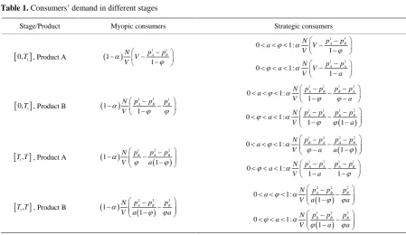
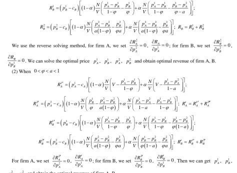
av−p . Consumers’ demand in the different stages is shown in Table 1.According to consumers’ different demand for product A, B, we can obtain revenue function of firm A, B. (1) When 0< < <a
ϕ
1(
)
(
)
1 1 1 11 1 1 ;
1 1
A B A B
A A A
p p p p
N N
R p c V V
V V α α ϕ ϕ − − = − − − − + − −
(
)
(
)
1(
2 2)
1 2(
2 2)
2 2 1 2
1 ;
1 1
B A B B A A B
A A A A A A
p p p p p p p
N N
R p c R R R
V a V a a
α α
ϕ ϕ ϕ ϕ
− − −
= − − − − + − − − = +
[image:2.595.86.536.457.717.2]
Table 1. Consumers’ demand in different stages
Stage/Product Myopic consumers Strategic consumers
[ ]
0,T1 , Product A ( )1 1 1 1 A B p p N V V α ϕ − − − − 1 1 0 1: 1 A B p p N a V V ϕ α ϕ −
< < < −
− 1 2 0 1: 1 A A p p N a V V a
ϕ α −
< < < −
−
[ ]
0,T1 , Product B ( )1 1 1
1
1
A B B
p p p
N V α ϕ ϕ − − − −
1 1 1 2
0 1: 1
A B B A
p p p p
N a V a ϕ α ϕ ϕ − −
< < < −
− −
( )
1 1 1 2
0 1:
1 1
A B B B
p p p p
N a V a ϕ α ϕ ϕ − −
< < < − − −
[
T T1,]
, Product A ( ) ( )1 2 2
1
1
B A B
p p p
N V a α ϕ ϕ − − − − ( )
1 2 2 2
0 1:
1
B A A B
p p p p
N a
V a a
ϕ α
ϕ ϕ
− −
< < < − − −
1 2 1 1
0 1:
1 1
A A A B
p p p p
N a V a ϕ α ϕ − −
< < < − − −
[
T T1,]
, Product B ( ) ( )2 2 2
1
1
A B B
p p p
N
V a a
α ϕ ϕ − − − − ( )
2 2 2
0 1: 1
A B B
p p p
N a
V a a
ϕ α
ϕ ϕ
−
< < < − −
( )
1 2 2
0 1: 1
B B B
p p p
N a
V a a
ϕ α
ϕ ϕ
−
< < < − −
(
)
(
)
1 1 1 1 1 1 21 1
1 ;
1 1
A B B A B B A
B B B
p p p p p p p
N N
R p c
V V a
α α
ϕ ϕ ϕ ϕ
− − −
= − − − − + − − −
(
)
(
)
(
2 2)
2(
2 2)
22 2 1 ; 1 2
1 1
A B B A B B
B B B B B B
p p p p p p
N N
R p c R R R
V a a V a a
α α
ϕ ϕ ϕ ϕ
− −
= − − − + − = +
− −
We use the reverse solving method, for firm A, we set
2 2 0 A A R p ∂ =
∂ , 1 0 A A R p ∂ =
∂ ; for firm B, we set
2 2 0 B B R p ∂ = ∂ , 1 0 B B R p ∂ =
∂ . We can solve the optimal price p1A, 1 B
p , 2 A
p , 2 B
p and obtain optimal revenue of firm A, B.
(2) When 0< < <
ϕ
a 1(
)
(
)
1 1 1 21 1
1 ;
1 1
A B A A
A A A
p p p p
N N
R p c V V
V V a
α α ϕ − − ′ = − − − − + − −
(
)
(
)
1(
2 2)
1 2 1 12 2 1 ; 1 2
1 1 1
B A B A A A B
A A A A A A
p p p p p p p
N N
R p c R R R
V a V a
α α
ϕ ϕ ϕ
− − −
′= − − − − + − − − ′ = ′+ ′′
(
)
(
)
1 1 1 1 1 1(
2)
1 1
1 ;
1 1 1
A B B A B B B
B B B
p p p p p p p
N N
R p c
V V a
α α
ϕ ϕ ϕ ϕ
− − −
′ = − − − − + − − −
(
)
(
)
(
2 2)
2 1(
2)
22 2 1 2
1 ;
1 1
A B B B B B
B B B B B B
p p p p p p
N N
R p c R R R
V a a V a a
α α
ϕ ϕ ϕ ϕ
− −
′= − − − + − ′ = ′+ ′
− −
For firm A, we set
2 2 0 A A R p ′ ∂ =
∂ , 1 0
A A R p ′ ∂ =
∂ ; for firm B, we set
2 2 0 B B R p ′ ∂ =
∂ , 1 0
B B R p ′ ∂ =
∂ . Then we can get p1A, 1 B
p ,
2 A
p , p2B, and obtain the optimal revenue of firm A, B.
4. Numerical Experiments and Parameter Analysis
(1) When 0< < <a
ϕ
1, we set V =20, cA=5, cB =4, α =0.6,ϕ
=0.8. Assuming variable a changeswithin this range
(
0, 0.8)
, we do sensitivity analysis for variable a.From Figure 1, we can know consumer’s buying decision order is 1
A , B1, A2, B2, price satisfies
1 1 2 2
A B A B
p >p > p > p . When a reduces, price 2 A
p and 2 B
p increases. Consumer’s utility of buying product B in the first stage is larger than buying product A in the second stage. Consumers are more willing to buy product B, thus price of product B is priced higher.
(2) When 0< < <
ϕ
a 1, other assumptions remain unchanged, we set a=0.8. Assuming variable ϕ changes within this range(
0, 0.8)
, we do sensitivity analysis for variable ϕ.From Figure 2, we can know consumer’s buying decision order is 1
A , 2
A , 1
B , 2
B , price satisfies
1 2 1 2
A A B B
p >p > p > p . While ϕ increases, consumers’ willingness to buy product B enhances, consumers’ de-mand for product B increases and prices of manufacturer B in both two stages increase. In order to curb con-sumers turn to buy the product of firm B, firm A would reduce the price of product A in the second stage.
In Figure 3, when 0< < <
ϕ
a 1,ϕ
=0.7, when there exists strategic consumers, both firms’ revenue de-crease. Profit difference between firm A and B increases when α increases. When there exist strategic con-sumers in the market, firm B suffers more loss.5. Conclusion
[image:3.595.73.548.86.432.2] [image:3.595.98.520.240.426.2]Figure 1. Effect of a on price p.
Figure 2. Effect of ϕ on price p.
and consumer valuation decreasing coefficient determine the order of consumer’s purchase decision. Meanwhile, consumers’ strategic behavior affects both the two firms’ revenue, both firms have profit loss. And the firm who provides lower-quality products suffered more loss than that one who provides high-quality products.
References
[1] Granot, D., Granot, F. and Mantin, B. (2010) A Dynamic Pricing Model under Duopoly Competition. Manuscript, University of British Columbia, Canada.
[2] Levin, Y., McGill, J. and Nediak, M. (2009) Dynamic Pricing in the Presence of Strategic Consumer and Oligopolistic Competition. Management Science, 42, 291-293.
[3] Levin, Y., McGill, J. and Nediak, M. (2010) Optimal Dynamic Pricing of Perishable Items by a Monopolist Facing Strategic Consumers. Management Science, 19, 40-60.
[4] Dasci, A. and Karakul, M. (2009) Two-Period Dynamic versus Fixed-Ratio Pricing in a Capacity Constrained Duopoly.
European Journal of Operational Research, 197, 945-968. http://dx.doi.org/10.1016/j.ejor.2007.12.039
[5] Chen, Y.X. and Zhang, Z.J. (2009) Dynamic Targeted Pricing with Strategic Consumers. International Journal of In-dustrial Organization, 27, 43-50. http://dx.doi.org/10.1016/j.ijindorg.2008.03.002
[6] Li, H., Xiong, Z.K. and Peng, Q. (2010) Dynamic Price Competition for Two Parallel Flights with Passenger prefe-rence. Industrial Engineering, 13, 86-90.