Seismic Correction in the Wavelet Domain

SEISMIC CORRECTION IN THE WAVELET DOMAIN

Thesis by

Andrew A Chanerley

In Partial Fulfilment of the Requirements

for the Degree of

Doctor of Philosophy (by Publication)

May 2014

CONTENTS

Acknowledgments 4

Abstract 5

List of Figures 6

List of Symbols 8

Preface 9

Chapter 1 De-coupling of the Instrument Response from Legacy Records 1 Introduction 12

Some Theoretical Background to Seismic Instruments 2.1 A simple accelerometer model 14

2.2 Some Instrument Parameters 15

2.3Digital accelerometers 17

3 Instrument de-convolution with standard methods 20

3.2Time domain de-convolution of instrument response 21

3.2 Frequency domain de-convolution of instrument response 23

3.3 Pre-filtering the Convolved Data

4.0 De-convolution of unknown instrument characteristics using adaptive algorithms 28

4.1 Summary of De-Convolution with the QR-RLS and the TLS algorithms 30 Inverse QR-Recursive Least Squares (QR-RLS) algorithm 30 The Total Least Squares (TLS) 31

6 Results 41 6.1 Some results from Chi-Chi Event, Taiwan (1999), stations TCU052, TCU068

and TCU129 41

6.2 Station TCU129 Chi-Chi Event (1999) 46

6.3 Some Permanent Displacement and tilt estimate summaries 51

7 Conclusions 53

References 54

APPENDIX I

Pseudo code for the un-decimated wavelet transform with de-noising 60

APPENDIX II 61

1. Chanerley, A. A., Alexander, N. A. “Using a Total Least Squares approach for Seismic Correction of Accelerometer Data”, Advances in Engineering Software.

Volume 39, Issue 10, pp 849-860, ISSN: 0965-9978, 2008

2. Chanerley, A. A., Alexander, N.A. “Correcting Data from an unknown

Accelerometer using Recursive Least Squares and Wavelet De-noising”, Computers and Structures, Issue 21-22,85 1679-1692, Nov 2007

3. Chanerley, A. A., Alexander, N. A.“Novel Seismic Correction approaches without instrument data, using adaptive methods and de-noising”, 13th World Conference on Earthquake Engineering, Vancouver, Canada, paper 2664, August 1st-6th, 2004.

4. Chanerley, A. A., Alexander, N.A. “An Approach to Seismic Correction which includes Wavelet de-noising”, Proc of the 6th International Conference on Computational Structures Technology ISBN 0-948749-81-4, , Prague, Czech Republic, paper 44, 4-6th Sept, 2002. doi:10.4203/ccp.75.44

5. Chanerley, A. A., Alexander, N.A., Berrill, J., Avery, H., Halldorsson, B., and Sigbjornsson, R. “Concerning baseline errors in the form of acceleration transients when recovering displacements from strong motion records using the undecimated wavelet transform”, Bulletin of the Seismological Society of America, vol. 103, pp. 283-295, February, 2013, doi: 10.1785/0120110352

6. Chanerley, A. A., Alexander, N.A., ”Obtaining estimates of the low-frequency ‘fling’, instrument tilts and displacement time series using wavelet decomposition”,

Bulletin of European Earthquake Engineering, vol. 8, pp231-255, 2010

7. Chanerley A. A., Alexander, N A, Halldorsson, B, 'On fling and baseline correction using quadrature mirror filters', 12th International Conference on Civil,

Structural and Environmental Engineering Computing, paper 177, Madeira, Portugal,

1-4 September, 2009 "doi:10.4203/ccp.91.177

8. Chanerley A. A., Alexander, N A., ‘Automated Baseline Correction, Fling and Displacement Estimates from the Chi-Chi Earthquake using the Wavelet Transform’9th International Conference on Computational Structures Technology

Athens, Greece, 2-5th _{Sept., 2008 http://dx.doi.org/10.4203/ccp.88.197}

Acknowledgements

This study and research would have not been possible were it not for the support of a list of people, both internal and external to the University.

To the Grace of God, the Lord Jesus Christ, that I survived two major and life-threatening operations during this research and study period, lived to tell the tale and to complete the publications.

To my wife for her love, support and encouragement.

Dr Nicholas Alexander, Civil Engineering Dept., University of Bristol, colleague, friend and mentor with whom the whole study began, over a lunch and some discussions on the processing of seismic data.

Dr Wada Hosny, my Director of Studies at UEL, whose constant encouragement and support along the way is gratefully acknowledged and appreciated

Professor Ragnar Sigbjornsson, Dr Benedikt Halldorsson, Dr Simon Olafsson, of the Earthquake Engineering Research Centre (EERC), in Selfoss, Iceland. In particular for their warm welcome during my visits to the EERC and the many useful and informative discussions over lunch in the Cafe Krús. In particular though the sharing of data after the Mw6.3, 29th May, 2008 earthquake in the SISZ, which produced

conference papers and a journal paper based in part on the Mw6.3, 29th May data.

Dr John Berrill, Dr Hamish Avery from the Canterbury University Seismic Project (CUSP) for generously providing information on their CUSP seismograph. Their seismograph made an impact in harnessing a wealth of data from the Mw7.1,

September 4th _{2010, Darfield Event in Christchurch, New Zealand. The many email}

Abstract

List of Figures

Figure 1 CUSP 3B Digital Accelerograph, Canterbury Seismic Instruments Ltd 18 Figure 2 Frequency response curves for Instrument correction methods 22

Figure 3 Classical Single Degree of Freedon System (SDOF) instrument

characteristics. The bold line is a typical value for the instrument SMA-1, with an

instrument damping ratio γ = 0.6 24

Figure 4: Comparison of estimate displacement time-series (for 1999 Chi-Chi

event, station TCU068N) using various correction schemes 27

Figure 6 Adaptive RLS diagram 29

Figure 7 Comparison of QR-RLS recovered filters and original "unknown" FIR test

filter (Kanai-Tajimi accelerogram 33

Figure 8 Comparison of extracted instrument characteristic from the El-Centro (1940) event using (i) QR-RLS adaptive filter and wavelet pre-denoising

(ii) SDOF instrument response ( f =10Hz,ξ =0.552) 34

Figure 9 Frequency and phase response plots for a 7-coefficient TLS inverse filter.

The event is TAI03.150N from the SMART-1 Array in Taiwan. 36

Figure 10 Frequency and phase response plots for a 9-coefficient TLS inverse filter. The event is TAI03.150N from the SMART-1 Array in Taiwan 36

Figure 11 A 4- channel, analysis (decomposition) wavelet filter bank

showing sub-band 40

Figure 12 TCU052NS LFS, fling, which shows results before (red, green) and after

(blue) baseline correction, wavelet used is the bior1.3 42

Figure 13 TCU052EW low-frequency sub-band, fling, which shows results before (red) and after baseline correction (blue). The wavelet used is the bior1.3 43

Figure 14 Recovered tilt gθacceleration, velocity and displacement response of

instrument A900 for the TCU052 component 44

Figure 15 The resultant plots for TCU052EW after the corrected low frequency sub-band (LFS) are added to the high frequency sub-band (HFS) 44

Figure 16 TCU068NS low-frequency sub-band 45

Figure 17 Acceleration Tilt transient for TCU068NS 46

Figure 18 TCU129EW, low-frequency sub-band fling 47

Figure 21 low and high frequency sub-bands for TCU129NS 49

Figure 22 low frequency sub-band vertical component TCU129V 50

Figure 23 LFS, HFS, and Corrected for TCU129V 50

Table 1 Some typical analogue and digital instrument characteristics 17 Table 2 Summary of zero velocity points employed and estimated peak tilt

acceleration 51

Table 3 Comparison of residual displacement (wavelet method) vs GPS 52 Table 4 Comparison of residual displacement (wavelet method) vs GPS 52

List of Symbols

u(t) : signal in time

H(ω) or H(f) : Fourier transform of h(t) U(ω) : Fourier transform of u(t)

E(ω) : Fourier transform of ‘noise’ DR: Dynamic Range

x : recorded instrument response ω : natural frequency

γ : critical damping

ψi : angle of rotation of ground surface about x, y, and z {i=1,2,3}

ag : ground acceleration

T : sampling interval

h : vector of filter coefficients d : vector of a desired signal a : recorded acceleration R : upper triangular matrix

Q : unitary matrix (also used for Householder Matrix) 0 : null matrix

P : inverse correlation matrix λ : ‘forgetting’ factor

Preface

This thesis is based on a summary of the papers published below in international scientific journals or in the proceedings of international conferences. The list is not exhaustive, but contains the papers as summarised in this thesis.

The structure of the thesis is in three chapters and its approach follows a historical description. Chapter 1 begins with the first part of the research, which was to obtain better estimates of ground motion from recorded seismic data by de-coupling the instrument response, where unfortunately and in most cases, the instrument characteristics were not available to facilitate the de-coupling. The approach was to treat the problem as one of system identification applying adaptive algorithms which iterated to an optimal description of the inverse instrument response.

Chapter 2 then continues on to the main part of the research with a summary of the wavelet transform method developed to recover the low-frequency acceleration fling pulse such that integration can proceed to the velocity pulse and the displacement fling-step. The novel method uses the undecimated wavelet transform with de-noising which is effective in removing frequency noise, but without removing the low-frequency signal. This is one of the key issues that render the method a success.

The link between the chapters and papers is broadly the limitation of the various instruments used with which to record the seismic data. These limitations therefore have required the development of novel algorithms with which to overcome some of the problems associated with instrument inadequacy in order to extract useful data. This thesis addresses some of the problems and summarises the formulated novel solutions.

The author of this thesis is the principal author of the papers listed below.

1. Chanerley, A. A., Alexander, N. A. “Using a Total Least Squares approach for Seismic Correction of Accelerometer Data”, Advances in Engineering Software.

Volume 39, Issue 10, pp 849-860, ISSN: 0965-9978, 2008

2. Chanerley, A. A., Alexander, N.A. “Correcting Data from an unknown Accelerometer using Recursive Least Squares and Wavelet De-noising”, Computers and Structures, Issue 21-22,85 1679-1692, Nov 2007

3. Chanerley, A. A., Alexander, N. A. “Novel Seismic Correction approaches without instrument data, using adaptive methods and de-noising”, 13th World Conference on Earthquake Engineering, Vancouver, Canada, paper 2664, August 1st -6th, 2004.

4. Chanerley, A. A., Alexander, N.A. “An Approach to Seismic Correction which includes Wavelet De-noising”, Proc of The Sixth International Conference on Computational Structures Technology ISBN 0-948749-81-4,Prague, Czech Republic, paper 44, 4-6th _{September, 2002 doi:10.4203/ccp.75.44}

6. Chanerley, A. A., Alexander, N.A., ”Obtaining estimates of the low-frequency ‘fling’, instrument tilts and displacement time series using wavelet decomposition”,

Bulletin of European Earthquake Engineering, vol. 8, pp231-255, 2010

http://dx.doi.org/10.1007/s10518-009-9150-5

7. Chanerley A. A., Alexander, N A, Halldorsson, B, 'On fling and baseline correction using quadrature mirror filters', 12th International Conference on Civil,

Structural and Environmental Engineering Computing, paper 177, Madeira, Portugal,

1-4 September, 2009 " doi:10.4203/ccp.91.177

8. Chanerley A. A., Alexander, N A., ‘Automated Baseline Correction, Fling and Displacement Estimates from the Chi-Chi Earthquake using the Wavelet Transform’9th International Conference on Computational Structures Technology

Chapter 1 De-coupling of the Instrument Response from Legacy

Records

1

Introduction

The structural/geotechnical engineering analyst/designer needs a complete set of boundary conditions (i.e. ground accelerations, velocities and displacements) at every location a structural artefact makes contact with the ground. A full spatiotemporal ground motion description is required rather than just ground accelerations at a single point. For this however a statistically significant sample of strong motion records is needed so that behaviour can be confidently predicted for unknown and critical future seismic events. However a statistically significant sample is the first problem we face i.e. the dearth of data, we do not have all the ground motion data we need. That is to say we do not have enough recordings for every location type and magnitude combination. There is insufficient good quality data so as not to neglect some of the older time histories recorded with analogue instruments. There are now arrays of instruments in the USA and Japan, but of course the problem is still with us because clearly the earthquake still has to occur within range of the instruments provided.

Data of ground motion acceleration recorded during seismic events is important to the process of developing models of system behaviour. Reliable, error free, experimental data is a major factor in the scientific method of developing and validating theoretical models. In the case of earthquake engineering ground motion times-series are used to predict the performance of structural systems to seismic events. As computational power increases the employment of non-linear time-history analysis of structural artefacts, e.g. buildings, bridges, etc. has become more feasible and widespread. These very challenging numerical models are subject to many unknowns; such as non-linear material behaviours. However, the greatest of these unknowns come from the loading, i.e. the ground motion, acceleration time-series, velocity pulses in the near and far field and displacement fling steps.

of freedom nor do they record velocities or displacements. The advent of satellite global positioning means that if accelerographs are coupled with GPS then it is possible to obtain some information about ground displacements. However, the sampling rate and dynamic range associated with GPS is generally low so this limits the frequency bandwidth of information that can be obtained. Nevertheless, more information is always required and a bonus.

Classically, structural engineers have avoided the problem of ground motion displacements by formulating their analyses in terms of a moving coordinate frame. That is we consider structural accelerations, velocities and displacements relative to the moving ground [17]. In this formulation the resulting equations of motion can be written in terms of ground motion acceleration alone. Nevertheless, for the most part, we still neglect the unrecorded ground rotational accelerations. This approach is reasonable for the case where the structure is small, i.e. less that 25m in length horizontally, [18]. Observed wavelengths of ground motion displacement may not impose any significant differential displacement on small structures. For longer, larger structures, i.e. very large buildings, bridges, tunnels, pipelines and dams, differential seismic displacements are more credible.

However, as has been already stated, we do not directly record ground motion displacement time-series. At first glance it appears that acceleration can be simply integrated twice to obtain displacement. While this is true in principle, in practice noise in the recording is the problem. Low frequency noise caused by the unrecorded ground rotations destroys any reasonable estimate of the true ground motion displacement time-series obtained by double integration. This is in part due to modern digital instruments not being 6-axis instruments, so a complete picture of ground motion acceleration, velocity and displacement at a point is not possible.

frequency (i.e. less than 0.1Hz) fling pulse is buried in low-frequency noise. Thus, it is difficult to remove the low frequency noise without removing the low-frequency ‘fling’ when applying standard filtering methods. In [3, 20] the reported permanent displacement of the ground during the Chi-Chi, Taiwan (1999) event was some 10m (reported by GPS). Compare this with an estimated (imposed) zero value in permanent displacement obtained by using a cut filter “correction”. Clearly low-cut filtering can produce very large errors in estimated ground displacements.

In this thesis we review published procedures for processing and correcting accelerograph data. The generic theoretical background to both analogue and digital instruments is considered as are the sources of noise/error along with the effect of ground rotations on accelerograph performance. The thesis reviews various techniques for noise/error reduction. The thesis also discusses the vexed problem of obtaining estimates of ground motion displacement time-series from accelerograph data.

2

Some Theoretical Background to Seismic Instruments

2.1 A simple accelerometer model

A strong motion instrument, commonly termed an accelerograph, is one that can be viewed as a generic process h t( ) that transforms an input signal (e.g. the actual ground motion) u t( ) into some output signal (e.g. the recorded ground motion) v t( ), thus

( )

( ) (

)

( )

v t ∞ h τ u t τ τ ε t

−∞

=

∫

for mathematical simplicity. This equation (1) can be re-expressed in the frequency domain as following linear equation

( )

( ) ( )

( )

V ω =H ω U ω + Ε ω (2)

where U( )ω , V( )ω and Ε( )ω are the Fourier transforms ofu t( ), v t( ) and ( )t

ε respectively and H( )ω is the Fourier transform ofh t( ). Any instrument should

record the signalv t( ), which should be a very good estimate of u t( ) i.e. ideally H( )ω would equal one and Ε( )ω zero.

2.2 Some Instrument Parameters

The first Strong motion recordings were obtained in Long Beach in 1933, [21]. The first accelerographs were optical-mechanical instruments that produced traces of ground acceleration on paper or film. These were analogue instruments, for example such as Kinemetric’s SMA-1 used in USA, SMA-C and DC-2 accelerographs used in Japan, these were widespread until the mid 1980s when digital instruments began to be used. In fact these instruments were still in situ in the late 1990s because they were considered relatively maintenance free and up front purchase costs had already been met. The problems with these analogue instruments and their subsequent legacy recordings were:

(i) The dynamic range of analogue accelerographs was relatively low. The

dynamic range DR where:

DR =20 log(max | ( ) | / min | ( ) |)v t v t , (3)

Where min | ( ) |v t _{and max | ( ) |}v t are the smallest and largest amplitudes that can be recorded. Usually the dynamic range is usually expressed in decibels (dB):

For analogue instruments this dynamic range was limited by the breadth of the recording paper/film and the width of the trace line, for example recordings made on recording paper have a maximum amplitude of about 10cm and a minimum resolution of 0.1mm, i.e. a DRdB = 60dB, or 3 orders of magnitude.

Thus, these instruments are subject to large quantization errors [23] and this was particularly a problem for very small events where little of the dynamic range was employed. Full scale on analogue accelerographs, max | ( ) |v t , was typically 1g and this is a problem in the case of very large seismic events as it resulted in clipping of peaks (similar to arithmetic saturation in digital instruments) of the signal.

(ii) The frequency bandwidth of analogue accelerographs was low. The bandwidth was limited by the instruments natural frequency. The optical-mechanical instruments behaved like a low-pass filter, attenuating all components of the recorded signal a little above the instruments natural frequency. In the 1930-40’s the operation frequency bandwidth was ~ 0-20Hz that improved over time to ~ 0-80Hz [24]. The bandwidth was in practice never down to DC as low frequency, so called baseline, errors where difficult toeliminate. This was because digitization of analogue paper/film records resulted in low frequency noise that was difficult to eliminate, though often attempted [6].

(iv) The threshold acceleration (the trigger) used to start the recording meant that all data ‘pre-trigger’ was normally lost. This sometimes resulted in the P wave arrival time being lost by this time delay.

(v) Digitization of analogue paper/film records resulted in much lower signal to noise ratio (SNR) than that of modern digital instruments. The so called baseline errors caused by low frequencies resulted in very large problems in the accurate determination of low frequency ground displacements time-series. In some legacy recordings erroneous spikes are found caused by errors in the automated digitization process. This was highlighted in [11] and shown to have a significant effect of derived acceleration response spectra.

It is clear therefore that there are number of problems surrounding legacy recording. Correction of these records is discussed in later sections of the paper but it worth noting that some care should be taken when employing these recording in engineering analysis.

Table 1: Some typical analogue and digital instrument characteristics

2.3 Digital accelerometers

Digital instruments are superior to the older analogue instruments in terms of performance. For example the digital recording system at each ICEARRAY station in

Name Dynamic Range Full

Scale Range

Signal to Noise Ratio

Operational Bandwidth

Ref.

CUSP 3B 80 dB 4g 91 dB DC to 80Hz [25]

CUSP 3E 120dB 3g 130dB DC to 80Hz [25]

130-SMA 113dB 4g ~166dB DC to 100Hz [26]

ETNA 108 dB 4g ~114dB DC to 200Hz [27]

Iceland (Figure 1) and the stations in CanNet, New Zealand, comprises a low-cost, single unit, CUSP-3Clp strong-motion accelerographs manufactured by Canterbury University Seismic Project in New Zealand, for the Canterbury Seismic Network in New Zealand. The units are equipped with 24-bit, tri-axial, low-noise (~70 µg rms) Micro-Electro-Mechanical (MEM) accelerometers with a high maximum range (± 2.5 g) and a wide-frequency pass-band (0-80 Hz at a 200 Hz sampling frequency) [63, 64]. These instruments have an amplifier, an anti-alias filter, a 24-bit A/D convertor and memory. Table 1 gives typical examples of dynamic range, full scale range, SNR’s and operational bandwidths of some modern digital accelerometers with a SMA-1 analogue accelerometer as a comparison. The dynamic range of the 24-bit digitizer is 6.02*23 ≈139dB, each additional bit increasing the dynamic range by20log₁₀

( )

Figure 1: CUSP 3B Digital Accelerograph, Canterbury Seismic Instruments Ltd

base (for the case where a large array of instruments are deployed [28]) and are coupled with GPS sensors that are able to determine position before and after a seismic event.

While digital accelerometers are superior to their analogue counterparts they are still only 3 axis instruments. Moreover some of the earlier digital instruments had internal filters, which removed the low frequency noise, but also removed any low-frequency, pulse-like accelerations, which cause the displacement fling-steps. That is to say they only record translational accelerations and not rotational accelerations. The assumption being that ground rotations (the commonly referred to tilts – pitch, roll and yaw) are small enough to be neglected. These are small in most cases, but in fact their effects can be considerable when velocity and displacement need to be recovered.

The effects of tilting are discussed in [2, 4, 13, 44, and 45] in particular in the long period which leads to dc shifts in velocity and offsets in the final displacement. Moreover [1] has demonstrated displacement offsets by using numerical simulations, a tilt of 0.1o (1.75mrad) is added to the Hector Mine seismic data. This gave displacement offsets similar to those obtained in the seismic data analysed and published and shown in this thesis for the TCU068NS station of the Chi-Chi (1999) event. The simulations in [1] showed a similar permanent displacement when Hector Mine was contaminated by a simulated tilt as that for the actual data from the recorded TCU068 station. It is shown in [3, 4] above that after operating on the seismic data using the wavelet transform method, the angle of tilt can be estimated.

The approximate equations [1, 3] which describe small tilt angles are as follows:

Longitudinal x₁ +2ω₁γ₁x₁ +ω₁2x₁ =−ag₁ + gψ₁ (5)

Transverse x₂ +2ω₂γ₂x₂ +ω₂2x₂ =−ag₂ +gψ₂ (6)

Vertical x₃ +2ω₃γ₃x₃ +ω₃2x₃ = −a_g3 (7)

γ = critical damping,

g = acceleration due to gravity,

ψ = rotation of the ground surface about x axis

ag = ground acceleration.

The conclusions from the above equations are that the two horizontal sensors are responding to horizontal acceleration and tilts and that the vertical sensor is responding to vertical acceleration only. Clearly there is an “error” in the recorded horizontal ground motion that is present even for the case of digital instruments. This error is an unknown, time varying, functiongψ_i, where i=

{ }

translational components and i=3 is the vertical component. [3] suggested that this error produces a signal to noise ratio, for the 1999 Chi-Chi TCU068 record, of around 31dB. This value is clearly far lower than the instrument signal to noise ratio as in Table 1. As an example of the effect tilts can have on the double time integration of the acceleration record then a displacement offset of 100cm over 100sec, requires a tilt angle of 20.4 x 10-6radians. Chapter 2 of the thesis dealing with recovery of displacements shows the considerable offsets created by small and abrupt changes in acceleration.

3

Instrument de-convolution with standard methods

recorded relative displacement response, an instrument correction can be applied as follows:

( )

( )

( )

( )

ag

2

2γω −ω

− −

=   (8)

where γ is the viscous damping ratio, ω is the transducer's natural frequency and

( )

a_g is the ground acceleration. The above expression (8) can be used to

de-convolve the recorded motion from the ground acceleration in either the time [6,9,29] or frequency domain [7,61].

3.1 Time domain de-convolution of instrument response

Analogue instruments such as the SMA-1 have their own dynamic response characteristics that affect their recording. This instrument response is classically modelled by a single degree of freedom system [7] (i.e. a simple small oscillation pendulum) as shown in equation (1). One wave to de-convolve the instrument response is to do so in the time domain as follows below.

Applying the central difference [6, 9] to equation (8) and using the approximation [9]

that the values of the acceleration of the uncorrected accelerograms are −ω_n2x(t)

gives a 3-tap FIR convolver for−(ω2T2)a_g(t), where T is the sampling rate of the digitised accelerograms, as:

4 2

2 2 2

2

) 4 2 ( ) 4

4 1 (

4 = + + − + ₋ + ₋

−

= T a_g T T a_i T a_i a_i

y ω γω ω γω (9)

where now a_i−n =−ω2x_i−nare the discrete values of the instrument acceleration output of the uncorrected accelerograms. For values of γ=0.6, f =25Hzand

600 / 1 =

T the expression becomes:

4 2 0.38046

72386 . 0 10432 .

0 = − ₋ + ₋

−

= ag ai ai ai

y (10)

2 1 2

2 2

2

) 1

( 2 ) 2

1

( + + − + ₋ + ₋

= −

= T ag T T ai T ai ai

y ω γω ω γω (11)

For values of γ =0.6, f =25Hzand T =1/600 the expression becomes:

2 1 0.43211

5975 . 0 2962 .

0 = − ₋ + ₋

−

= ag ai ai ai

y

(12)

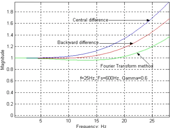
Figure 2: Frequency response curves for Instrument correction methods

3.2 Frequency domain de-convolution of instrument response

Equation (8) can also be transformed into the frequency domain [7, 29] by applying the Fourier transformation

) ( ) (f A f H

g

X =− where

   

 

      +      

− =

i

i f

f i f

f f

H( ) 1 2γ (13)

where the approximate acceleration output of the instrument is A(f)=ω2X(f). The ground acceleration in time can therefore be recovered from the inverse Fourier transform of the ground accelerationX_g(f), obtained from the Fourier transform of

0 0.2 0.4 0.6 0.8 1 1.2 1.4 1.6 1.8 2 100

0.2 0.4 0.6 0.8 1

Freq ratio (ω/ω₀)

A

m

pl

itude,

|H

|

0 0.2 0.4 0.6 0.8 1 1.2 1.4 1.6 1.8 2 -1

-0.8 -0.6 -0.4 -0.2 0

0.2 0.4 0.6 0.8

1

Freq ratio (ω/ω₀)

P

has

e,

ar

g(

H

) /π

Instrument natural frequency Instrument damping

Figure 3 Classical Single Degree of Freedon System (SDOF) instrument characteristics.

The bold line is a typical value for the instrument SMA-1, with an instrument damping ratio γ = 0.6

This instrument characteristic (nonlinear frequency response function) is displayed in the above Figure 3. As the instrument’s ratio of critical damping increases the effect of the instrument resonance attenuates, so producing a flatter instrument response. Consider the bold line highlighted in the figure that corresponds to 60% percent of critical damping. This instrument’s characteristic is relatively flat for frequencies below the instruments natural frequency ω0. The phase of H_i( )ω is also displayed

and appears almost linear for frequencies below the instruments natural frequency ω0

at this value of damping. A linear phase change results in a constant time-shift in the time-domain was considered fairly neutral. Thus, is easy to understand the choice of ratio of critical damping of 0.6 that was used for SMA-1. However, by modern standards this response is far from flat and the phase distortion (though almost linear) does require some correction. This correction can be achieved in the time-domain as suggested by [7] or simply by using the FFT, IFFT and equations (13) and as suggested by [10].

natural frequency). Recovering the true ground acceleration requires de-convolution therefore in correcting for the instrument characteristic we end up amplifying the higher frequency terms (as shown in the frequency responses of Figure 2) that have been attenuated by the instrument. Therefore high frequency noise and alias errors, together with higher frequency signal components, will be amplified. Instrument correction in this case should be followed by a high cut filter to attenuate again the high frequency noise/signal.

3.3

Pre-filtering the Convolved Data

Any process that converts an analogue signal into a digital one runs the risk of introducing aliasing errors. Discrete sampling of a continuous signal at a sampling rate f resultsin a digital signal is unable to distinguish components above the Nyquist frequency f/2 [23]. Furthermore, frequency components above this Nyquist limit may produce errors in the sampled signal cause by high frequency components folding back power below the Nyquist frequency. So aliasing error is an issue whether an A/D converter is used (for digital seismographs) or some optical-mechanical digitization (for analogue seismographs). To mitigate this error, an anti-alias filter is employed in the case of digital seismographs and this filter is a simple high-cut filter that seeks to remove frequency components above the Nyquist frequency, this filter precedes the A/D converter. Unfortunately for the case of an analogue seismograph the aliasing errors have already been introduced through the optical-mechanical digitization device. Therefore, a high-cut filter appears unnecessary as it cannot remove the aliasing errors after they have been folded back into the low frequency bandwidth. Nevertheless, this high-cut filter may still have utility. If it is employed after the instrument correction (as in [8, 10]) it can mitigate the amplification of instrument noise at frequencies above the natural frequency of the instrument. This effectively removes the least reliable part of the signal.

quadratic de-trending of the data (i.e. finding the least square linear or quadratic fit and then subtracting this from the recording) or (ii) to use of some low-cut filter. These two processes are qualitatively similar as both are, in effect, low-cut filters. If a low-cut filter is to be employed we would favour one that has known and designed filter characteristics i.e. one with a known corner frequency, flat pass-band and zero/linear phase characteristic and so method (ii) rather than (i) is preferable.

Many digital accelerometer transducers are reliable down to DC so technically there should not be any baseline error. Once the true ground motion acceleration time-series is obtained it is typical to try and obtain both the ground velocity and displacement time-series.

0 10 20 30 40 50 60 70 80 90 -2000

-1500 -1000 -500 0 500 1000

time [s]

D

is

pl

ac

em

ent

[

c

m

]

0 10 20 30 40 50 60 70 80 90

-400 -200 0 200 400

TCU068N

A

c

c

. [c

m

/s

2]

raw low-cut filter 0.02Hz low-cut filter 0.05Hz low-cut filter 0.1Hz

Piecewise linear detrend,(breakpoints 25s,60s) Corrected (wavelet based) Chanerley & Alexander

Figure 4: Comparison of estimate displacement timeseries (for 1999 chi-chi event,

station TCU068N) using various correction schemes

This problem of amplification of low frequency noise (by a double-time integration filter) was well known and tackled almost universally by some low-cut filter with a cut-off frequency <0.25Hz, e.g. the Ormsby filter [30], which is a Finite Impulse response filter (FIR) [31, 32], was a popular filter to use in the early days of correction procedures. The corrected records in the PEER strong motion database [19] filters it’s data. The trouble with this approach is that it eliminates signal components with the noise at the very low frequency. Figure demonstrates how sensitive this low-cut filtering can be. There are clear differences in the estimated ground displacement obtained by a Butterworth zero-phase (IIR) [31, 32] filter at 0.02Hz, 0.05Hz and 0.1Hz (cut-off frequency).

displacement) that is present after the strong ground motion. That is to say that often the estimated residual displacement from a low-cut filter record is often near to zero. Thus, it implies that there is never any residual ground deformation after an earthquake and GPS readings have shown this to be clearly incorrect.

Obtaining reliable ground displacement estimates from older analogue data is very problematic because of the presence of large noise (caused by misalignments in paper/film processing) so low-cut filtering here is only to stabilise the acceleration time-series. For these cases, the displacement time-series thus obtained are highly questionable. For modern recordings (from digital instruments) the removal of the very low frequency of the time-series is also questionable as it removes important parts of the signal. This problem is considered in Chapter 2 of the thesis.

4.0 De-convolution of unknown instrument characteristics using

adaptive algorithms

The de-convolution of legacy instrument response (i.e. its non-flat frequency response) discussed in the beginning of section 3 makes a number of assumptions. Firstly, we assume to form of the instrument response (filter), in this it is defined by a single degree of freedom system (for these optical-mechanical instruments). Secondly, we need to know the instrument parameters, namely its natural frequency and ratio of critical damping. Some legacy recordings have been obtained from accelerographs that may no longer exist and so it is not possible to validate either of these two assumptions exactly. Thus, we are left with a system identification problem i.e. the determination of the characteristic or footprint that the instrument leaves imposed on the time-series. Once obtained the resulting inverse filter can be applied to the data in order to de-convolve the instrument response. The actual ground acceleration a_gand the accelerometer system g are unknown, and the adaptive

algorithm estimates an optimal system to improve the ground motion estimate, see Figure 6.

Unknown system

g

+

-

εk

Σ Delay

Adaptive algorithm

h=

ga

g ag*=

Figure 6 Adaptive RLS diagram

In the time domain, the actual ground acceleration a_g is convolved “*” with the filter

function of the accelerometerg to give the recorded signala.

g a

a= _g* (14)

In this thesis, the implementation of the adaptive algorithm attempts to find a solution to the inverse problem, equation (2) where ideally the inverse filter h is such that

1

−

=g

h and then the desired signal dequals the actual ground motion a_g.

d h

a* = (15)

Solution of this problem, in general, is not possible; however under certain limited condition it is possible to produce an estimate of h from the recorded signala. The conditions for the application of the recursive least squares method is that a and a_g

4.1 Summary of De-Convolution with the QR-RLS and the TLS

algorithms

There are many different, but related, least squares algorithm for obtaining a system identification. The Least Mean Square (LMS) algorithm [42] is the simplest and easiest adaptive algorithm to implement. However, its performance, in terms of computational cost and fidelity, is not as good as the Recursive Least Square (RLS) [43] and Square Root RLS algorithms (QR-RLS) [12, 43]. There also exists the total least square (TLS) [13]. The QR-RLS and TLS successfully obtained estimates of the instrument response from just the output of the accelerograph during earthquakes in Taiwan and Iceland. The basis for the QR-RLS algorithm and the TLS are summarised.

Inverse QR-Recursive Least Squares (QR-RLS) algorithm

QR-decomposition-based RLS algorithm is derived from the square-root Kalman filter counterpart Haykin [42], Sayed [43]. The ‘square-root’ is in fact a Cholesky factorization of the inverse correlation matrix. The derivation of this algorithm depends on the use of an orthogonal triangulation process known as QR decomposition. _      = 0 R

QA (16)

Where 0 is the null matrix, R is upper triangular and Q is a unitary matrix. The QR

decomposition of a matrix requires that certain elements of a vector be reduced to zero. The unitary matrix used in the algorithm is based on a Givens rotation or a Householder reflection, which zero’s out the elements of the input data vector and modifies the square root of the inverse correlation matrix. The QR-RLS is as follows in equation (17) below.

Where P = the inverse correlation matrix, λ = forgetting factor, γ = a scalar and the gain vector is determined from the 1st column of the post-array. U(n) is a unitary transformation which operates on the elements of λ-1/2_uH_(n)P1/2_{(n-1) in the pre-array}

zeroing out each one to give a zero-block entry in the post-array. The filter coefficients are then updated commencing with equation (18), which is the gain vector. This is followed by equation (19) the a priori estimation error.

[

]

)

(n k n 1/2 n 1/2 n

k = γ− γ− (18) ε(n)=d(n)−hH(n−1)u(n) (19) h(n)=h(n−1)+k(n)ε(n) (20)

This is turn, leads to the updating of the least-squares weight vector, h(n), in equation (9). These inverse-filter weights are an estimate of the inverse transfer function of the instrument and these are then convoluted with the original seismic data in order to obtain an estimate of the true ground motion.

The Total Least Squares (TLS

)

The Total Least Squares [13, 62] has a history of applications in de-convolution in medicine and spectroscopy. It was applied to the de-convolution [13] of seismic data in order to obtain an estimate of the instrument response. This method of de-convolution has the advantage that it includes the error in the sensitivity matrix as well as the data vector. Essentially the problem is given by equation (21):

(

)

A

minimise x−b (21)

In some practical engineering situations the matrix A is in fact a function of the measured data, as is the case here. Therefore we need to take into account that noise measurements occur on both sides of the matrix equation. This is essentially a total least squares problem, where we have the matrix A plus noise and the matrix b plus noise, [A +E] and [b + r].

The Total LeastSquares (TLS) problem is formulated as follows:

r] [b

x E]

[A + ˆ = + (22)

Equation (22) can be re-written as:

(

[

] [ ]

The solution is obtained by first finding the SVD of [A|b]∈IRm×p as in (26); where

n m

R I

A∈ × ,p=n+1

T

V

Σ

U

b]

|

[A

=

] ... [

], ...

[u1u2 um = v1v2 vp

= V

U , Σ=[diag(σ₁,σ₂,...,σ_r)] (25)

where mm

R I ×

∈

U and V∈IRp×p are square orthogonal matrices, diagonal matrixΣ∈IRm×pwith non-negative number on the diagonal; it is the same size as

] b |

[A . One way to obtain a solution is to find a Householder matrix Q such that

   

  =

α

T

y

0 W Q

V (26)

then the minimum norm solution is given by

α

/

ˆ y

x=− (27)

4.2 Some Results for the QR-RLS and the TLS

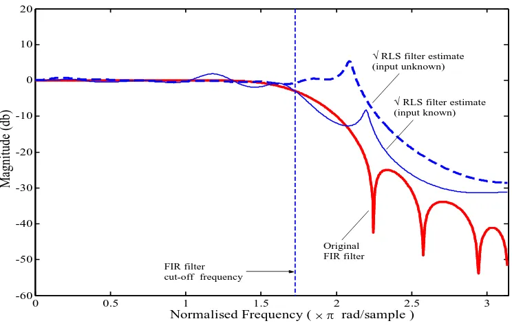
Figure 7 demonstrates the performance of the QR-RLS in recovering the frequency response of an “unknown filter” embedded in a simulation of an earthquake using the Kanai-Tajimi model. The simulation shows a reasonable estimate, in particular over the key flat region of the frequency response.

The plots of Figure 8 show that at low frequencies to approximately 40Hz for the El-Centro Eastern component the QR-RLS inverse filter show an approximately flat response (0dB) in the region of interest. The El-Centro Northern component is approximately flat to about 75Hz and the phase plots are approximately linear.

0 0.5 1 1.5 2 2.5 3

-60 -50 -40 -30 -20 -10 0 10 20

Normalised Frequency ( ×π rad/sample )

M

agni

tude

(db)

√ RLS filter estimate (input unknown)

Original FIR filter FIR filter

cut-off frequency

√ RLS filter estimate (input known)

Figure 7 Comparison of QR-RLS recovered filters and original "unknown" FIR test

100 101 102 -10

0 10 20 30 40

50 100 150 200 250 300

-100 -50 0 50 100 150 200

Frequency (Hz)

M

a

gni

tude

(

dB

)

El-Centro 1940-East El-Centro 1940-North

P

h

as

e (

D

eg

.)

Frequency (Hz) 2nd Order ODE Instrument Model

2nd Order ODE Instrument Model

El-Centro 1940-North

El-Centro 1940-East

Figure 8 Comparison of extracted instrument characteristic from El-Centro (1940) event using (i) QR-RLS adaptive filter and wavelet pre-denoising (ii)

SDOF instrument response ( f =10Hz ,ξ =0.552)

There is of course an element of uncertainty in both models, in particular given the instruments’ years in situ, whether the calibration parameters were in fact correct. The QR-RLS approach does perform quite well in the pass band region, which is, for the engineering, the region of interest. The RLS therefore provides a reasonable indication of instrument performance. These results demonstrate the usefulness of using the QR-RLS in order to de-convolve the instrument response without any prior knowledge of the instrument parameters.

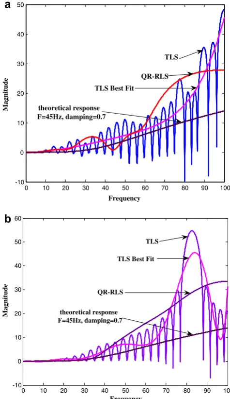
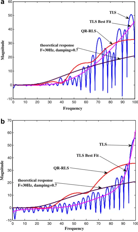
Figure 9 and Figure 10 with 7- and 9-coefficients respectively, from station

TAI03.150N (SA-3000 instrument) with a 25Hz anti-alias filter. Figure 9 and Figure 10 demonstrate that the TLS algorithm performs well and recovers the inverse response of the 5th order Butterworth, anti-alias filter, with a cut-off at 25Hz. The TLS algorithm secured the same cut-off frequency at 25Hz as shown in the frequency response plots for station TAI03.150N and also stations TAI03.149, TAI03.161 and the TAI03.170, all of which have the same anti-alias filter and showed similar performance and results. The phase plots are linear, which means that all the frequencies are impressed with a constant phase difference or the same time shift for all the data points in the time history. Once the inverse filter coefficients are recovered the data is then filtered through the same coefficients in order to obtain an estimate of the de-convoluted data. Results from events in Iceland using the SMA-1, A-700, DCA-333 and SSA-1 instruments with cut-off frequencies at 15Hz, 45Hz, 30Hz and 53Hz respectively as in [13] show that the performance of the TLS algorithm is provides good estimates of the cut-off frequencies in particular for the z-component, which is less sensitive to tilts than the x- and y- components.

0 0.2 0.4 0.6 0.8 1 -1500

-1000 -500 0

Normalized Frequency (×π rad/sample)

P

h

ase (

d

eg

rees)

0 0.2 0.4 0.6 0.8 1

-20 0 20 40

Normalized Frequency (×π rad/sample)

M

ag

n

it

u

d

e (

d

B

)

TLS instrument inverse filter frequency response:7-coeffs

Figure 9 Frequency and phase response plots for a 7-coefficient TLS inverse filter.

The event is TAI03.150N from the SMART-1 Array in Taiwan.

0 0.2 0.4 0.6 0.8 1

-1500 -1000 -500 0

Norma lize d Fre que ncy (×π rad/sample)

Ph

ase (

deg

rees)

0 0.2 0.4 0.6 0.8 1

-20 0 20 40 60

Normalized Frequency (×π rad/sample)

M

ag

ni

tu

de

(d

B)

TLS:instrume nt inve rse filte r fre que ncy re sponse : 9-coe ffs

Figure 10 Frequency and phase response plots for a 9-coefficient TLS inverse filter.

Chapter 2 The Recovery of Velocity and Displacement from the

Acceleration Time-Series and the Localisation in Time and Removal

of the Baseline Error

5.0 Introduction

Unfortunately recovering displacements from acceleration time-histories is not straight forward. Direct double integration does not yield a stable displacement time history as is shown in Figure 3. The displacement time histories in Figure 3 demonstrate the sort of linear and quadratic trends obtained from double integrating after filtering with standard low-cut filters with differing cut-off frequencies.

Sophisticated methods exist for correcting baseline errors and obtaining stable double time integration. Grazier [1,2,44,45] was the first to advocate a baseline correction procedure by obtaining and fitting a straight line to a segment of the velocity. Chiu in [46] high-pass filtered before integration, Iwan et al in [47] removed pulses and steps by locating the time points which exceeded a pre-defined acceleration, later generalized by Boore et al in [11,15,48,49]. Boore and Akkar [50] by added further time points and made the time point’s t1 and t2 free of any acceleration thresholds, the

accumulated effects of these baseline changes represented by average offsets in the baseline. Wu in [51] also used a modified a method due to [47] on the Chi-Chi event and defined t1 at the beginning of the ground motion, and defined t2 on the basis of a

flatness coefficient and defined a further parameter t3, the time at which the

‘fling’ pulse in time by the wavelet transform algorithm, is novel, never before having been recovered, though always inferred from some strong-motion time-series and modelled as a sinusoidal pulse.

The undecimated wavelet algorithm, described in detail in papers [3, 4, 20 and 56] uses the undecimated wavelet transform, with a de-noising scheme, which is the key to its success. The advantage of using the un-decimated transform with de-noising is that it is automated and it recovers the low-frequency ‘fling’ time history, locates an acceleration transient i.e. the baseline error and permits stable integration to displacement.

Generally the ‘fling’ contains an acceleration transient (‘spike’), which on integration shifts the DC level of the velocity and causes linear trends in displacement. It has been shown that the vertical component is insensitive to tilts, therefore any ‘spikes’ in the vertical direction in the acceleration time history are usually attributed to instrument noise and indeed are usually small when compared with the ‘spikes’ of the horizontal components, which are attributed to ground rotation. This use of the undecimated wavelet transform recovers the residual displacement and extracts and then removes ground rotation acceleration transients that are a cause of double-time integration problems. This shows its usefulness and flexibility in being able to provide not only displacements, but in addition information on the rotational acceleration transients, hitherto always inferred, but never located. We begin this chapter with de-noising

5.1 De-noising overlapping spectra using a threshold

particular filtering low-frequency noise will also filter the low-frequency signal (i.e. the fling) so is to be avoided.

The application of a de-noising scheme initially applies a soft threshold [16, 35, 38, 39 and 40] to both the low-frequency and higher frequency sub-bands signals after applying the wavelet filters. However, it was subsequently found that for some earthquakes applying a threshold to the higher frequency sub-bands removed too much detail in the de-noising process (Haldorsson 2009, private communication). Therefore the soft threshold initially applied to the higher frequency sub-bands was removed from the algorithm. This retained the detail without affecting the overall displacement result and when overlaying the original time history on the corrected time history, didn’t demonstrate any significant differences.

A soft threshold time-seriesa_i, wherei∈

{

}

(removed).

(

) ( )

i i i

i

i

a a a

a

a

τ τ

τ

 _{− >}

 = 

≤ 

 (3)

Typically the threshold τ is estimated from the standard deviation of the data σ , multiplied by Donoho’s “root two log N” [16, 38]

2 logN

τ σ= ,

6745 . 0

MAD

=

σ (4)

resilient to outliers in a data set than the sample standard deviation. In order to use MAD as consistent estimator for the standard deviation, it is divided by a scale factor that depends on the probability distribution of the noise (which is again unknown). For a normal distribution this scale factor is Φ−1_{(3/4) = 0.6745, where Φ}−1 _{is the}

inverse of the cumulative distribution function for the standard normal distribution, and hence equation (4)

5.2 A note on the un-decimated wavelet transform

From an engineering and seismological perspective, the easiest way to envisage the wavelet transform is in terms of octave filters. These are quite common in digital audio. Octave filters form the basis of the wavelet transform, whether the transform is decimated or un-decimated. The wavelet transform comprises in this case well designed filter banks [33, 34, 35, 36, 37]. The decimated, discrete wavelet transform (DWT) is applied in an octave-band filter bank, implementing successive low-pass and high-pass filtering and down sampling by a factor of 2, so that every second sample is discarded. As an example, a 4-channel filter bank scheme is shown in Figure (11). The filters used in wavelet filter banks are digital finite impulse response filters (FIR), also called non-recursive filters because the outputs depend only on the inputs and not on previous outputs.

H(ω)

1 2 3 4

ω/8 ω/4 ω/2

4 (Gx) x LP

Hx 3 G(Hx)

2 (G(H(Hx)) 1 (H(H(Hx))

Figure 11: A 4- channel, analysis (decomposition) wavelet filter bank showing sub-band

HP 2

LP 2

HP 2

LP 2

HP 2

However, there is a problem with the DWT in that due to down-sampling the DWT it is not shift-invariant. Aliasing can occur between the sub-bands, which is undesirable if the application needs de-noising as in this case. Therefore the easiest way to overcome this is not to down-sample so that the length of the signal remains constant and not as in the decimated DWT and so we use a generalization of the DWT, which is the un-decimated wavelet transform or stationary wavelet transform (SWT), which is shift-invariant. Since we don’t decimate then instead we have to interpolate by pushing zeros into each level of the transform (i.e. between the filter coefficients) i.e. dyadically up-sampling, this is the á trous algorithm [37, 41] (trous = holes). It was also shown in [38 and 39] that the SWT de-noises with a lower root-mean-square error than that with the standard DWT and de-noising is a key requirement for this application. Furthermore, the inverse SWT (iSWT) averages the estimates at each level again minimizing the noise, so overall the SWT is a better transform to apply. Time domain filter banks in Figure (11) show the SWT, there are also the iSWT synthesis filter banks for reconstruction. In the analysis filter banks the easiest thing to do is to push zeros (á trous) in between the filter coefficients and keep filtering even and odd samples from every band. In the synthesis filter banks they are averaged at each level. The data of course is also de-noised between the analysis phase using the SWT and the synthesis phase using the iSWT. The appendix presents some pseudo code in order to illustrate how the undecimated wavelet transform with de-noising is constructed.

6 Results

6.1 Some results from Chi-Chi Event, Taiwan (1999), stations

TCU052, TCU068 and TCU129

integration of the transient. These are precisely the error offsets observed in the velocity and displacement time histories after double-time integrating the (almost) sinusoidal acceleration time history of Figure 12. It is inferred that acceleration transient of 3.015cm/s/s is in fact a gθ tilt transient. The area of the acceleration tilt profile is 7.21cm/s, which is the velocity offset. Similarly the area under the velocity step is 294.7cm, the maximum displacement offset as shown in Figure 12. The corrected displacement is 641cm, which compares with those of other researchers, the GPS reading is 845cm. The point to note is that the area of the acceleration transient is exactly equal to the constant velocity offset after integrating the acceleration transient and observed in the velocity sub-band. Then after integrating the constant velocity offset, then the result matches exactly the linear trend in the displacement before correction. The TCU052EW low frequency, fling time-histories are shown in Figure 13. In this case the acceleration tilt transient occurs at 40.06s, approximately 8s earlier than the NS component. The displacement is -352cm (GPS -342cm) the instantaneous tilt acceleration gθ, shown in Figure 14, is 12.96cm/s/s and θ the instantaneous tilt angle is 13.2mrads. The area of the acceleration tilt profile is 2.98cm/s, the velocity offset.

0 10 20 30 40 50 60 70 80

-20 0 20

[cm/s

2 ]

TCU052N

0 10 20 30 40 50 60 70 80

0 50 100

[cm/s

]

0 10 20 30 40 50 60 70 80

0 200 400 600 800

[cm]

time [s]

Figure 12: TCU052NS LFS, fling, which shows results before (red, green) and after

0 10 20 30 40 50 60 70 80 -20

0 20

[cm/s

2 ]

TCU052E

0 10 20 30 40 50 60 70 80

-60 -40 -20 0

[cm/s

]

0 10 20 30 40 50 60 70 80

-400 -200 0

[cm]

time [s]

Figure 13: TCU052EW low-frequency sub-band, fling, which shows results before (red)

and after baseline correction (blue). The wavelet used is the bior1.3

0 10 20 30 40 50 60 70 80 90 -10

0 10 20

cm/s/s

Tilt Acceleration, velocity dc offset, displacement linear trend

0 10 20 30 40 50 60 70 80 90

-10 0 10 20

X: 90 Y: 2.966

cm/s

0 10 20 30 40 50 60 70 80 90

-100 0 100 200

X: 90 Y: 180.7

time /sec

c

m

Max linear trend = 180.7cm Area = 180.7 cm

inst acceleration = 12.96cm /s/s

velocity dc offset = 2.97cm /s Area = 2.97cm /s

Figure 14 Recovered tilt gθ acceleration, velocity and displacement response of instrument A900 for the TCU052EW component

0 10 20 30 40 50 60 70 80 90

-500 0 500

TCU052E

[c

m

/s

2

]

0 10 20 30 40 50 60 70 80 90

-200 0 200

[c

m

/s

]

0 10 20 30 40 50 60 70 80 90

-500 0 500

[c

m]

time [s]

Figure 15 The resultant plots for TCU052EW after the corrected low frequency

sub-band (LFS) are added to the high frequency sub-sub-band (HFS)

Similar results are obtained for TCU068NS in Figure 16 and Figure 17, using the undecimated wavelet transform method, the peak instantaneous tilt angles calculated from the peak acceleration transient are calculated as -6.9mrad (-6.75cm/s2_{) (EW) and}

12.09mrad (11.86cm/s2). It is these peak acceleration transients, which are inferred as due to instantaneous tilt/rotation angles, that cause the dc shift in velocity in the latter portion of the time history and prevent stable double-time integration. These results are similar to those in [53] using a different method, with which to estimate the tilt angles. The estimates of displacement are shown in Table 5.

0 10 20 30 40 50 60 70 80

-50 0 50

[cm/s

2 ]

TCU068N

0 10 20 30 40 50 60 70 80

-50 0 50 100 150

[cm/s

] _{X: 90}

Y: 11.61

0 10 20 30 40 50 60 70 80

0 500 1000

[cm]

time [s]

Figure 16 TCU068NS low-frequency sub-band, fling, which shows results before (light

gray) and after (black) baseline correction. The triangular area in the acceleration is the

0 10 20 30 40 50 60 70 80 90 0

5 10

[cm

/s/

s]

TCU068NS, Tilt acceleration transient, velocity dc shift and displacement offset

X: 45.65 Y: 9.565

0 10 20 30 40 50 60 70 80 90

0 5 10 15

[cm

/s] X: 90

Y: 11.62

0 10 20 30 40 50 60 70 80 90

0 200 400 600

X: 90 Y: 504.7

Time /sec

[c

m

]

Area = 11.62cm/s

Area = 504.7cm

Figure 17 Acceleration Tilt transient for TCU068NS at 45.65s. The resulting constant

velocity dc shift of 11.61cm/s is a clear example of a post shaking, flat velocity time

history

6.2 Station TCU129 Chi-Chi Event (1999)

0 10 20 30 40 50 60 70 80 -10

0 10

[cm/s

2 ]

TCU129E

0 10 20 30 40 50 60 70 80

0 10 20 30

[cm/s

]

0 10 20 30 40 50 60 70 80 90

0 50 100

[cm]

time [s]

Figure 18 TCU129EW, low-frequency sub-band fling before (red) and after (blue)

baseline correction showing tilt/rotation in acceleration and baseline dc shift in velocity

0 10 20 30 40 50 60 70 80 90

-5 0 5

cm/s/s

Tilt Acceleration, velocity dc offset, displacement trend

0 10 20 30 40 50 60 70 80 90

-10 0 10

cm/s X: 90

Y: -8.815

0 10 20 30 40 50 60 70 80 90

-500 0 500

time /sec

c

m _{X: 90}

Y: -392 Area = 8.82cm/s

Area = 392 cm

0 10 20 30 40 50 60 70 80 90 -1000

0 1000

TCU129E

[cm/s

2 ]

0 10 20 30 40 50 60 70 80 90

-100 0 100

[cm/s

]

0 10 20 30 40 50 60 70 80 90

-50 0 50 100

[cm]

time [s]

Figure 20 low frequency sub-bands (red), high frequency sub-bands (black), Corrected

(blue) using bior1.3 for TCU129EW component obtained at level 9

then zeroes-out the acceleration from 28.1s and re-integrates to give the corrected time histories shown below in Figure 21. The GPS displacement for the NS component was -32.1cm that obtained using the presented wavelet transform method is -26.8cm. The TCU129V component is interesting because it suggests either at least 9 more tilts, or just a very noisy instrument. However, in [15] there is a suggestion that the location of the instrument (A900) on a concrete pier may have been the cause of the oscillatory ringing. Certainly there are significant oscillatory effects as can be seen from the time history in Figure 22.

0 10 20 30 40 50 60 70 80 90

-1000 0 1000

TCU129N

[cm/s

2 ]

0 10 20 30 40 50 60 70 80 90

-50 0 50

[cm/s

]

0 10 20 30 40 50 60 70 80 90

-50 0 50

X: 90 Y: -26.28

[cm]

time [s]

Figure 21 low frequency sub-bands (red), high frequency sub-bands (black), corrected

(blue) using bior 2.6 for TCU129NS component obtained at level 9

0 10 20 30 40 50 60 70 80 -10

0 10

[cm/s

2 ]

TCU129V

0 10 20 30 40 50 60 70 80

-10 0 10

[cm/s

]

0 10 20 30 40 50 60 70 80 90

-20 0 20

X: 90