The design and performance of non-linear vibration
isolating materials.
COLLIER, Paul.
Available from Sheffield Hallam University Research Archive (SHURA) at:
http://shura.shu.ac.uk/19492/
This document is the author deposited version. You are advised to consult the
publisher's version if you wish to cite from it.
Published version
COLLIER, Paul. (1985). The design and performance of non-linear vibration isolating
materials. Doctoral, Sheffield Hallam University (United Kingdom)..
Copyright and re-use policy
* V — ■ J_* aJi_* if* a K Y | POND STREET , SH E FFIE L D S I 1W B )
(Q
7 D |100
424
501
7
TELEPENlllllllllllllllll
Sheffield City Polytechnic Library
REFERENCE ONLY
37
iMf
iO-25 %
cs.>r
& r c ? W
u o 4 - >
L b ( v \
^ - C O p ^ v 22jfcH5
, 5 ' . ^ I
3
h[
14
^
ProQuest Number: 10694373
All rights reserved
INFORMATION TO ALL USERS
The qua lity of this reproduction is d e p e n d e n t upon the qua lity of the copy subm itted.
In the unlikely e v e n t that the author did not send a c o m p le te m anuscript and there are missing pages, these will be noted. Also, if m aterial had to be rem oved,
a n o te will in d ica te the deletion.
uest
ProQuest 10694373
Published by ProQuest LLC(2017). C o pyright of the Dissertation is held by the Author.
All rights reserved.
This work is protected against unauthorized copying under Title 17, United States C o d e M icroform Edition © ProQuest LLC.
ProQuest LLC.
789 East Eisenhower Parkway P.O. Box 1346
T H E D E S I G H A N D P E R F O R M A N C E OF N O N - L I N E A R V I B R A T I O N ISOLATING MATERIALS
by
PAUL COLLIER BSc
A thesis submitted to the Council for National Academic Awards in partial fulfilment of the requirements for the
degree of Doctor of
Philosophy-Sponsoring Establishment : D e p a r t m e n t of A p p l i e d Physics, S h e f f i e l d City Polytechnic
Collaborating Establishments : Bruel and Kjaer (UK) Ltd. JCB reaearch Ltd.
r,v< rO-YT[C«Wc'4A' .. 2\>,.
4 Y ( p ^ o . [ \ % ^ >
{ C °
__s___
THE DESIGN AND PERFORMANCE OF NON-LINEAR VIBRATION
ISOLATING MATERIALS
by P COLLIER
ABSTRACT
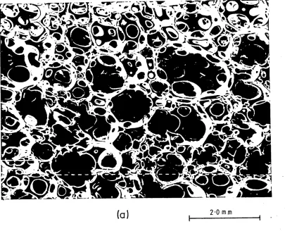
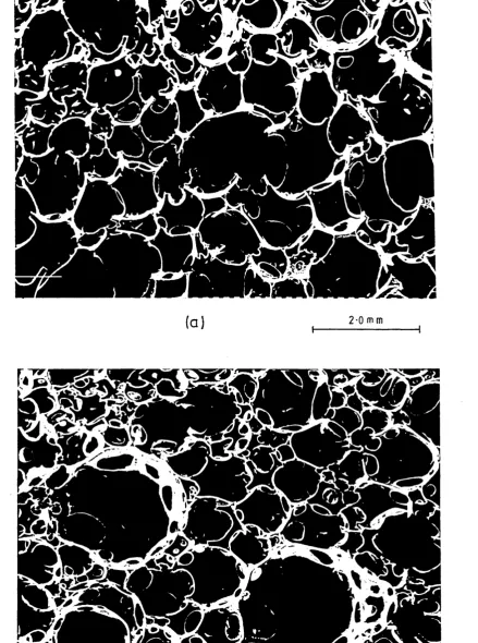
The m e c h a n i c a l p r o p e r t i e s of r e s i l i e n t c e l l u l a r materials, such as dynamic stiffness and damping, depend on s e v e r a l p h y s i c a l p a r a m et er s c h a r a c t e r i s t i c of the m a t e r i a l and the c on di ti on s of use, eg p er me ab i l i t y , elastic modulus, cellular structure, static pre-strain. In many end use situ at io ns the p r e - c o m p r e s s i o n s and dynamic amplitudes are large and the material operates in a non-linear regime. The effects of non-linear material behaviour on the performance of systems employing cushion foams has not previously been reported on.
In thi s w o r k the i n f l u e n c e of n o n - l i n e a r m a t e r i a l behaviour on the vibration isolation characteristics of the m a t e r i a l is examined. P r e v i o u s t h e o r e t i c a l and experimental studies have been confined to small strain conditions where the material behaves in a linear fashion and the properties are independent of deformation. This work extends the theoretical analysis to allow the study of the v a r i a t i o n of the m e c h a n i c a l p r o p e r t i e s and v i b r a t i o n i s o l a t i o n p e r f o r m a n c e with pre-strain. The f luid f lo w m od el prop os e d by Gent and R usch is shown to be inadequate and an alternative proposed which conforms closely to experiment. This is extended to non-Newtonian fluids and incorporated in a model for fluid flow damping in the non-linear regime.
T H E D E S I G N A N D P E R F O R M A N C E OF N O N - L I N E A R
VIBRATION ISOLATING MATERIALS
CONTENTS i
ACKNOWLEDGEMENTS iv
PUBLICATIONS AND PRESENTATIONS v
LIST OF SYMBOLS vi
1. INTRODUCTION 1
2. THE MICROPROCESSOR CONTROLLED DYNAMIC MECHANICAL SPECTROMETER
2.1 General Considerations 7
2.2 The Complete Spectrometer 8
2 . 3 Electrical Hardware
2.3*1 Digital Excitation Output Interface 12
2.3*2 Memory Mapped Input ADC Interface 17
2.3*3 Signal Conditioning Circuits 21
2.3*4 Transducers 25
2.4 The Measurement Algorithm
2.4*1 Theoretical Treatment 27
2.4*2 Numerical Methods 28
2.4*3 Errors Arising in the Algorithm 31
2.4*4 Mass Compensation System 33
2.5 The Control Software
2.5*1 Program Structure 38
2.5*2 High Level Data Analysis 40
2.5*3 Machine Code Routines 46
2.6 The Mechanical Mounting System 49
2.7 Testing and Calibration
2.7*1 System Calibration 54
2.7*2 System Performance Checks 57
3. T H E A I R - F L O W C H A R A C T E R I S T I C S OF C E L L U L A R
MATERIALS
3.1 I n t r o d u c t i o n 6 0
3 . 2 T h e o r e t i c a l T r e a t m e n t 63
3 . 2 . 1 V i s c o u s L a m i n a r F l o w 6 4
3 . 2 . 2 I n e r t i a l F l o w 69
3 . 3 E x p e r i m e n t a 1 C o n s i d e r a t i o n s 7 0
3 .4 R e s u l t s a n d D i s c u s s i o n
3.4.1 Z e r o - S t r a i n P r o p e r t i e s 79 3 . 4 . 2 S t r a i n D e p e n d e n t B e h a v i o u r 8 9
3 • 5 T h e o r e t i c a 1 E x t e n s i o n to I n c l u d e the F l o w of M o n - N e w t o n i a n F l u i d s t h r o u g h C e l l u l a r M a t e r i a l s
3.5.1 Z e r o - S t r a i n B e h a v i o u r 95 3 . 5 . 2 E f f e c t of P r e - S t r a i n on the N o n - N e w t o n i a n
P e r m e a b i l i t y 9 9
4 . THE EFFECT OF COMPRESSIVE PRE-STRAIN 01 DYNAMIC PROPERTIES
4.1 T h e S m a l l S t r a i n D y n a m i c P r o p e r t i e s i n t h e A b s e n c e of F l u i d - F l o w E f f e c t s
4 .1.1 I n t r o d u c t i o n 101
4 . 1.2 E x p e r i m e n t a l M e t h o d 1 0 8 4.1 .3 R e s u l t s a n d D i s c u s s i o n 1 1 4
D y n a m i c
S y s t e m s M e c h a n i c a l P r o p e r t i e s of L i q u i d - F i l l e d
4.2.1O R e v i e w of N e w t o n i a n F l u i d - F l o w P r o c e s s e s 1 29
J
•
CO• T h e o r e t i c a l T r e a t m e n t of N o n - N e w t o n i a n
F l u i d F l o w D a m p i n g 1 3 6 4 .2.3 E x p e r i m e n t a l D e t a i l s 146 4 .2 . 4 R e s u l t s a n d D i s c u s s i o n 1 5 2
5. THE RESPONSE OF NON-LINEAR VIBRATION ISOLATORS
5 • 1 S m a l l S t r a i n A m p l i t u d e D ^ n a m i _ c B e h a v i 0 u r , A p p l i e d 10 t h e P r o b l e m 0 f V e h i c l e S e a t i n g a n d D y n a m i c R i d e C o m f o r t
5.1.1 I n t r o d u c t i o n 1 7 4
5 * 1 . 2 M u l t i - D e g r e e o f F r e e d o m P e r s o n - S e a t
M o d e l l i n g 1 8 2
5 . 1 . 3 C o m p a r i s o n o f P r e d i c t e d R e s p o n s e to
F i e l d M e a s u r e m e n t s 1 9 0
5.1.4 The I n c l u s i o n of F lu id F l o w D a m pi n g
Processes in the cushion material 198
5*2 The Response of a^ Non-Linear Vibration Iso lating System To Large Amplitude Oscillatory Motion 5.2.1 Introduction
5.2.2 Review of Chaotic Motion 5.2.3 Experimental Determinations
6. CONCLUSIONS AND FUTURE WORK
6•1 Air-Flow Properties of Cellular Plastics
6.2 The Effects of Compressive Pre-Strain on Dynamic Properties
6.3 The Behaviour of Non-Linear Vibration Isolators 6.4 Future Improvements to the Spectrometer System
REFERENCES
APPENDICES
I) Summary of the S p e c i f i c a t i o n s of the Dynamic Mechanical Spectrometer.
II) Pascal Source Text for the Spectrometer Control Programs CONTROL, CALIBRAT and ANALYSIS.
Ill) F l o w C h a r t s for the M a c h i n e C o d e Routines in the S p e c t r o m e t e r s C on tr o l System.
IV) A s s e m b l e r List in g of the M a ch i n e Code Ro ut in es in the S p e c t r o m e t e r s C on t r o l System.
V) The H o o k e - J e e v e s N o n - L i n e a r S e a r c h Optimisation Technique 203 208 214
232
236
243250
252 1-1I I - 1
III-1
IV-1
ACKNOWLEDGEMENTS
The author wishes to express his a p p r e c i a t i o n to Dr N C H ilyard , Dr C M Care and Dr H M K o h l e r for s u g g e s t i n g
this research topic and for their guidance throughout the investigation. The author would also like to thank the c o l l a b o r a t i n g e s t a b l i s h m e n t s ; Bruel and Kjaer (UK) Ltd for the loan of equipment and the transfer of ideas, and
JCB R e s e a r c h Ltd for the loan of their v e h i c l e seat systems and s ug g e s t i n g the p ro gramme of work on the comfort of v e h i c l e operators. A p p r e c i a t i o n is also e x t e n d e d to a l l the s t a f f of the A p p l i e d P h y s i c s
d e p a r tm en t at S h e f f i e l d City P o l yt ec hn ic . P a r t i c u l a r thanks must go to; Dr J S Brooks and Mr M Furness for h e l p f u l advice, Mr J B e ad ma n for a s s i s t an c e with the m e a s u r e m e n t of the a i r - f l o w properties, Mrs G Sidda and Mr K B la ke for h e l p and a d v i c e with the SEM M i c r o s c o p e
facilities, and Mr G France, Mr T H u d s o n and Mr K Jaff re y for help with the construction of the dynamic mechanical spectrometer. Thanks is also due to Mr P S l i n g s b y and Mrs R Thomas of the Metallurgy Department for assistance
with the static testing of foam samples.
The author w o u l d also like to thank Brit is h V i ta Ltd, D u n l o p Ltd and BP C h e m i c a l s Ltd for p r o v i d i n g s u i t a b l e foams for testing.
PUBLICATIONS AND PRESENTATIONS
1 H i l y a r d N.C., C o l l i e r P., M c N u l t y G.J. & D o u g l a s D., 'Influence of seat cushions on vibrations in earth moving vehicles', Proceedings, Internoise '83, Edinburgh, Vol I, 527, July 1983.
2 M c N u l t y G.J., D o u g l a s D., H i l y a r d N.C. & C o l l i e r P., 'Vibr at ion in earth m o v i n g vehicles', Procee di ng s, Internoise '83, Edinburgh, Vol II, 913, July 1983*
3 Hilyard N.C., Collier P. & Care C.M., 'Dynamic Mechanical b e h a v i o u r of f l e x i b l e foam cushion m a t e r i a l s and its i n f l u e n c e on ride comfort', Proceedings, UK In fo rm al Group on Human Resp on se to Vibra ti on , N.I.A.E., Silsoe, Bedfordshire, September 1983.
4 H i l y a r d N.C., C o l l i e r P. & Care C.M., 'Influence of the m e c h a n i c a l p r o p e r t i e s of c e l l u l a r p l a s t i c c u h i o n m a t e r i a l s on ride c o m f o r t ’, Proceedings, 'Dynamics in A u t o m o t i v e E n g i n e e r i n g ' , C r a n f i e l d I n s t i t u t e of Technology, Bedford, p A.1 , April 1984
5 H i l y a r d N.C. & C o l l i e r P., ' Ef f e c t of v e h i c l e s ea t cushion material on ride comfort', Proceedings, 'Plastics on the road', London, p 6/1, D e c e m b e r 1 984*
6 Hilyard N.C. & Collier P., ' Response of a vibration isolator with distributed non-linear stiffness at large excitations', accepted for pub li ca t io n , J. Sound &
Vibration letters.
7 C o l l i e r P., N o r c l i f f e A. & H i l y a r d N.C., ' An u n d e r g r a d u a t e Case study to i l l u s t r a t e the role of computer aided m o d e l l i n g t e ch ni qu es in the c o n t r o l of vibration', Proceedings Fifth British Conference on the T e a c h i n g of V i b r a t i o n and N o i s e , S h e f f i e l d C i t y Polytechnic, p23-32, July 1985*
8 Care C., C o l l i e r P., H i l y a r d N.C., N o r c l i f f e A., R o dg er s G.G. & T h o m l i n s o n M.M., 'Improving d r i v e r comfort in m o t o r v e h i c l e s - a cas e s t u d y for A p p l i e d S c i e n c e
students', Proceedings, 2nd International Conference on the T ea ch in g of M a t h e m a t i c a l M o d e l l i n g , Exeter, J ul y 1985.
LIST OF SYMBOLS
A Boolean quantity, defined in table 2.2
A dc Component of input signals
A Area
A. (5x3) Matrix defined in equation 5.6 A c Surface area of cell
A 0 Effective cross-sectional area of sample
a Radius of pipe in section 3*5
a Curve fitting constant, defined in equation 4*8
ax ,ay,az Distances shown on figure 5*27
B Boolean quantity, defined in table 2.2
B (3x1) matrix defined in equation 5*6
B^ i = 1 , 00 A m p l i t u d e s of the h a r m on ic content in the input signals
B,B(e) Flow resistance coefficient
b Curve fitting constant in equation 4»8 b^ i = 1 , 00 Amplitudes of fourier series components _b Base point used in appendix V
C Boolean quantity, defined in table 2.2
C Curve fitting constant in equation 4*65 C Damping of a viscous element
C^,C2 »C^ Damping of human body subcomponents in figure 5»10 CQ C ri t ic a l damping of a lumped p ar am e t e r
spring-damper system
Cf Skin friction coefficient
Cm , Cn A m p l i t u d e s of input s ig n a l s at 50 Hz and 100 Hz C 0 Numerical constant in equation 3*5
C(n) Constant defined by equation 3«54 c Numerical constant in equation 3*2 c Constant in equations 5-25 and 5»27
i = 1 ,°° Amplitudes of fourier series components
D Radius of pipe d ia me te r to orifice d i a m e t e r in equation 3*5
D Curve fitting constant in equation 4.65
d Average cell diameter
d Diameter of orifice in equation 3*25
d-j ,d2 Loss tangents of the elements in the person-seat model of figure 5• 1 1
d^,d^(o)) Loss tangent of seat cushion in figure 5*11
dm Loss tangent of matrix d(w) Dynamic loss tangent
du/dr Shear rate
E^ Zero strain modulus of foam Eg Bulk modulus of gas
E r Modulus of solid polymer E^, E^(e) Storage modulus of matrix E^, E.{.(e) Transverse modulus of matrix
E(oj),E U ) Dynamic modulus, scalar and complex form
E'(w) Dynamic storage modulus
E"((jo) Dynamic loss modulus
e Fractional static pre-strain
e-^ Critical buckling strain, when T(e)=0.95
e-^ Strain when «(©) is minimum
emin Strain when T(e) is minimum e J Yield strain, when H(e)=0.95 _e^ Unit vectors in appendix V
F Force due to fluid flow
F Forcing function in equations 5*25-5.27
v Inertial force vector
F^ T o t a l f o r c e v e c t o r m e a s u r e d by the d y n a m i c mechanical spectrometer
f>|,f2 »f^ Resonance frequencies of human body components in figure 5*10
f(cot) Fourier series, defined in equation 4*54 G Gradient of line in figure 3*6
G(jd) Mean square variation used in appendix V
g ( z ) Restoring function used in equation 5*27
H Height of test piece
h^ Step lengths used in appendix V I Intercept of line in figure 3*6
Iq-I^ Integrals
Ij),In Coefficients defined in equation 5*11
Ix ,Iy,Iz Moments of inertia about the three axes
i Integer
5 A T
K Integer defined in equation 2.9
K,K(e) Permeability of matrix K(n),K(n,e) Non-Newtonian permeability
n,w) ,K(n,oo,e) Effective non-Newtonian permeability, defined by equation 4*38
K (go) , K (oo, e) Effective permeability, defined by equation 4*16
k Numerical constant
k^,k2 »k^ Stiffnesses shown on figure 5»34b
kx ,ky,kz Stiffnesses shown on figure 5*27 L Integer defined in equation 2.9
L Length of test piece
le Effective path length in matrix M Integer defined in equation 2.9
Masses of the elements in the person-seat model of figure 5*1 1
m Integer, chapter 2
m Hydraulic radius of voids in chapter 3
N Number of points sampled in one deformation cycle
n Fluid index
P Pressure
Pi_p^ Sample data point
P(w) Power spectrum, defined in equation 5*19
p Curve fitting constant, equation 4*8 j> Independent variables in appendix V
Q Volume flow rate of fluid
q Integer, chapter 2
q Curve fitting constant, equation 4*8 R Growth parameter used in equation 5*18
Resistances
Rp,Rjj Coefficients defined by equation 5*11 r Curve fitting constant, equation 4*10
r Radius
r Fluid flow fitting parameter defined in equation 4.61
S Area of orifice in equation 3*25
S,S(e) Netted surface area of matrix/ unit volume S-j-S^ Summations defined by equation 2.8
* * *
S-j,S2 »S^ S t if fn es s of the v i s c o e l a s t i c e l e m e n t s of the person-seat model of figure 5*11
S'-j,S'2 Storage stiffnesses in the person-seat model
Storage stiffness of the seat in the person-seat model of figure 5*11
T Time period of input signals
T(w) Transmissibility
t Time
tg Sampling time interval
u Linear flow velocity
u g Effective linear flow velocity
um Mean approach velocity
v Linear flow velocity, equation 3*1
v Curve fitting constant, equation 4-• 1 0
¥ Width of test piece
w Curve fitting constant, equation 4»10
X Q Vector displacement of sample
x Distance
x Co-ordinate axis in chapter 5, figure 5.22
Iterated population value in equation 5*18 x g Steady population value in equation 5.20
Y(jd) Function defined in appendix V
y Co-ordinate axis in chapter 5, figure 5.22
y(t) Input signal to mechanical spectrometer Z Amount of sample deformation. Displacement
•
Z Velocity in z direction
Z Acceleration in z direction
Z_ (3x1) matrix defined in equation 5*6
ZQ ,Zio Amplitudes of the displacements of the component masses in the 3-DOF person-seat model
Z,Z-| Vertical displacements in chapter 5
Z Displacements of the component masses in the 3-DOF person-seat model of figure 5*11
z Co-ordinate axis in chapter 5, figure 5»22
a Numerical constant in chapter 3
a a
a
Fluid flow parameter, compressible fluids Co-ordinate axis in chapter 5, figure 5*22
F e i g e n b a u m u n i v e r s a l constant = 2.5029, g i v e n in equation 5*22
3 Ratio of cell strut width to length, chapter 3 3 Co-ordinate axis in chapter 5, figure 5*22 3,3(e) Fluid flow parameter, incompressible fluids
r 1 ,r2 Coefficients, defined by equation 4-50
y Co-ordinate axis in chapter 5, figure 5.22
y,Y(e) F l u i d f l o w parameter, def in ed in e qu a ti o ns 4*14 and 4-44
Ymax Value of Y at the maximum damping frequency
Ap Pressure difference
Ax Thickness
A^ Quantity defined on figure 5*25
A(w) Coefficient defined in equation 4*36
6 Phase angle, equation 4*1
6 F e i g e n b a u m u n i v e r s a l constant = 4*6692, g i v e n in equation 5*21
6^ i = 1 ,°° Phase angle of input signal harmonics
^m»6n Phase a n g l es of input s i g n a l s at 50 Hz and 100 Hz e 9c(a)) Dynamic strain
£ Rate of change of dynamic strain = de/dt Quantity defined on figure 5*25
e 0 Dynamic strain amplitude
l^(u)) Coefficient defined in equation 4*36
r| Newtonian viscosity
D a Apparent viscosity, defined in equation 4*57 9 Phase angle in figure 2.12
0 Fluid flow fitting parameter, equation 4*61
A Dimensionless constant in chapter 3
y Zero shear rate viscosity for a power-law fluid
y F e i g e n b a u m u n i v e r s a l constant = 4.648, g i v e n by equation 5*23
V x ,Vy Parameters defined in equation 5.24
5(e) Dynamic storage modulus shape function, defined in equation 4*6
5(e)i Minimum value of 5(e)
B, Volume fraction of open cells
p Density
a Standard deviation
Of Stress due to fluid flow
am Stress due to deformation of matrix
Of Total stress from d e f o r m a t i o n of the m a t r i x and fluid flow
a(oo) ,a*{(d) Dynamic stress, scalar and complex form
T Tortuosity
x Stress due to fluid flow in a pipe, equation 3.28
T Stress at walls of pipe, equation 3*18
4 0 ,4(e ) Volume fraction of polymer
^>1 ,^2 Integral sums defined in equation 2.4
,^2 Coefficients defined by equations 4*21 and 4.22 T(e) Rusch shape function, defined by equation 4*6 T(e)m in Minimum value of T(e)
w Angular frequency
U)n R e s o n a n c e F r e q u e n c y of a 1 - D O F i s o l a t o r in equation 5*1
N a t u r a l f r e qu en cy of the 1-DOF i s o l a t o r in the vertical direction
0)x g F r e q u e n c y o f c o u p l e d o s c i l l a t i o n in the x and 3 directions, given by equation 5*24
1 . INTRODUCTION
R e s i l i e n t c e l l u l a r p l a s t i c s hav e w i d e s p r e a d p r a c t i c a l a p p l i c a t i o n s , s u c h as c o m f o r t c u s h i o n i n g , s h o c k
mitigation, v i b r a t i o n i s o l a t i o n and e nergy m a n a g e m e n t s y s t e m s . U n d e r the c o n d i t i o n s p r e v a i l i n g in m a n y applications, such as vehicle seating and packaging, the
c e l l u l a r matrix is often subject to large a m p l i t u d e deformations and large static (or quiescent) compressive deformation. Under these cond it io ns the m e c h a n i c a l p ro pe r ti e s of the m a t e r i a l are h i g h l y n o n - l i n e a r . The
i n f l u e n c e of these n o n - l i n e a r i t i e s on the v i b r a t i o n isolating performance of cushion foams has not previously been studied.
Earlier work on material behaviour by investigators such as Gent, Rusch and Hilyard, has led to a r e a s o n a b l e u n d e r s t a n d i n g of the m e c h a n i s m s g o v e r n i n g the dynamic
m e c h a n i c a l p r o p e rt i es of r e s i l i e n t c e l l u l a r pla st ic s. However the early experimental and theoretical studies w e r e c o n f i n e d , for the m o s t part, to s m a l l s t r a i n conditions where the response of the cellular material is approximately linear and to deformations about the
zero-strain condition. Small zero-strain conditions restricted the c o m p r e s s i v e d e f o r m a t i o n of the matr ix (both static and
practical applications.
During cyclic deformation of a flexible open-cell polymer foam two separate processes occur, one is associated with
the p o l y m e r m at r i x and the other a s s o c i at e d with f lu id e n c l o s e d by the matrix. Both of these p ro c es s es hav e been studied previously [eg 50,28], but both theoretical
and p r a c t i c a l work was r e st ri ct ed to s m a l l l e v e l s of
imposed static strain and Newtonian fluid flow.
Energy dissipation is an important feature of resilient c e l l u l a r p l a s t i c s in many a pp li ca ti on s. Three e ne rg y dissipation mechanisms operate. These are:
i) V i s c o e l a s t i c d a m p i n g p r o c e s s e s due to n o r m a l d e f o r m a t i o n s in the p o l y m e r f o r m i n g the c e l l u l a r structure. This process operates at both low and high levels of static compressive strain.
ii) Hysteresis associated with the catastrophic collapse of cell elements, which becomes important at high levels of compressive strain.
iii) F luid flo w p ro ces se s caused by the m ot i on of the
e n c l o s e d fluid through the c e l l u l a r matrix. This m e c h a n i s m w i l l operate at both low and high l e v e l s of
compressive strain and at frequencies determined by the foam and fluid in use and test piece geometry.
The r e l a t i o n s h i p between, and r e l a t i v e i m p o r t a n c e of these three processes in p a r t i c u l a r a p p l i c a t i o n s has
received little attention in the literature.
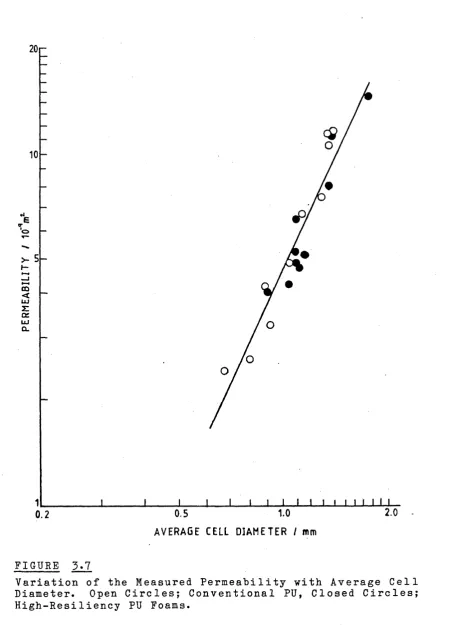
The permeability of the foam is an important factor when c o n s i d e r i n g d amping due to f luid flow. The f l o w of N e w t o n i a n fl ui ds t hrough c e l l u l a r s tr uctures has been
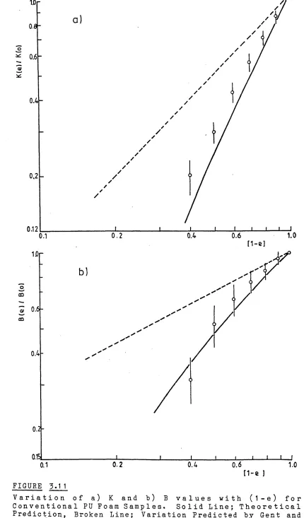
i n v e s t i g a t e d p r e v i o u s l y [28]. H o w e v e r the s i m p l i f i e d model treatments used have proved incapable of correctly p r e d i c t i n g the strain d e p e n de nc e of the f luid flow b eh av io ur . A t h e o r e t i c a l a n a l y s i s is p r e se nt ed in
Chapter 3 which uses a m o de l of the c e l l u l a r stru ct ur e based on flow through a packed bed. The predicted zero-strain and zero-strain dep en de nt a i r - f l o w p ro p e r t i e s are
c o m p a r e d w i t h e x p e r i m e n t a l d a t a and s h o w a b e t t e r c o r r e s p o n d e n c e t h a n e a r l i e r t r e a t m e n t s . R e c e n t
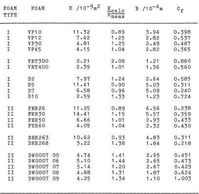
developments in foam manufacture technology have resulted in additives to control the fluid flow energy dissipation process and hence the vibration isolating characteristics of the material via changes in cellular structure [38]. A series of foams c o n t a i n i n g d if ferent amounts of the
vibration control additive have been tested in this work. The results have proved interesting and are summarised in chapter 3» An e xt en s i o n to the t h e o r e t i c a l m o d e l is presented here which includes the flow of a non-Newtonian f luid through the c e l l u l a r structure. The r e s u l t s of this study are used in C hapter 4 for the p r e d i c t i o n of
the f luid f lo w d amping p rocess with N e w t o n i a n and non-Newtonian fluid flow.
ene rg y d i s s i p a t i o n systems operate. The m o d u l u s and damping of the material are shown to be functions of the
imposed level of pre-compression. A study is presented, in Chapter 4, into the r e l a t i o n s h i p b e tw ee n the dynamic m e c h a n i c a l properties, and those measu re d using q u a s i s t a t i c l o a d i n g t e c h n i q u e s . It is s h o w n t ha t the e f f e c t i v e d y n a m i c s t i f f n e s s at a p a r t i c u l a r p r e compression is very different to the gradient of the F-D
curve at the same compressive strain.
For the case of the m e c h a n i c a l b e h a v i o u r of c e l l u l a r materials incorporating fluid flow processes, theoretical equations are developed which relate the observed dynamic
response to the physical properties of the material and the fluid. This t re atment f o l l o w s c l o s e l y that put forward by Gent and Rusch [39,74]. However in this case the work extends the treatment by considering the flow of incompressible non-Newtonian fluids and high levels of static deformation.
A major application of flexible cellular plastics is as vibration isolators. This type of material is commonly used in the c o n s t r u c t i o n of fu 1 1 - d e p t h v e h i c l e seat
cushions. In C hapter 5, a study is p r e se nt ed into the
v i b r a t i o n i s o l a t i o n c h a r a c t e r i s t i c s of n o n - l i n e a r c ellular plastic materials. The study is split into two s e c t i o n s , the f i r s t d e a l i n g w i t h s m a l l d y n a m i c e x c i t a t i o n s and the s e c o n d w i t h l a r g e d y n a m i c
excitations.
In the first section the application of vehicle seating is considered. This is imp or ta nt since since it is not
p o s s i b l e to s pecify a c ushio n foam p r o v i d i n g enhanced ride comfort unless the influence of cushion properties, eg s t i f f n e s s a n d d a m p i n g , on t h e v i b r a t i o n transmissibility of the person-cushion system is known. A multi degree-of-freedom model of the person-seat system is p r e s e n t e d and b e h a v i o u r p r e d i c t e d by the m o d e l
compared with responses of vehicle seats measured in the field. This m od el is much more c o m p l e x than those used by p r e v i o u s workers and good a gr ee me nt b e tw e e n p r e di c te d behaviour and that measured by other workers is obtained. The m od el studies are e xtended to show how f l u id f l o w
damping in the cushion material influences dynamic ride comfort. Another group of workers in this field have used the v i b r a t i o n c ontr ol a d d i t i v e d e s cr ib e d a b o v e to
influence the fluid flow process in the cushion material
and hence the vibration isolation characteristics. The
results of their experimental investigations do not fit a simple 1-DOF model incorporating fluid flow processes.
In the second section the response of a distributed non linear viscoelastic vibration isolator to large amplitude dynamic exci ta ti o ns considered. E x p e r i m e n t a l data iss'
presented which indicates that the classical theories of vibration isolation break down at high excitations. For a simple mechanical arrangement the motion of the isolated mass is found to be ver y c o m p l e x with c ou p l e d modes of
excitations the behaviour of the isolator system appears to exhibit the characteristics of chaotic motion [121]•
In order to measure the dynamic mechanical properties of the c e l l u l a r m a t e r i a l s o ve r the f r eq u e n c y range of interest, it has been n e c e s s a r y to des ig n and c on st ru ct an automated dynamic mechanical spectrometer suitable for the testing of 1 o w - s t i f f n e s s materials. The design of this equi pm ent is o u t l i n e d in Chapter 2. The system is
based around a c o m m e r c i a l l y a v a i l a b l e e l e c t r o m a g n e t i c e x c i t e r a n d a N a s c o m I I I m i c r o c o m p u t e r . T h e spectrometer operates over a frequency range of 0.07Hz to 1 OOHz and uses a novel measurement algorithm to determine the a m p l i t u d e and phase of the force and d e f o r m a t i o n s i g n a l s . The s y s t e m a l s o a l l o w s a u t o m a t i c m a s s compensation for the elements of the spectrometer between the f o r c e t r a n s d u c e r and the t es t p i e c e . A M a s s
compensation system which will operate at low frequencies is not a v a i l a b l e c o m m e r c i a l l y and is needed bec au se of the low stiff nes s of the test pieces used in this work. Operator control over all of the spectrometer's functions is achieved through an interactive microprocessor control system.
2. T H E M I C R O P R O C E S S O R C O N T R O L L E D D Y N A M I C M E C H A N I C A L SPECTROMETER
2.1 General Considerations
S e v e r a l systems are a v a i l a b l e c o m m e r c i a l l y for the m e a s u r e m e n t of the dynamic m e c h a n i c a l p r o p e rt ie s of resilient materials. The commercial systems investigated included the widely used Rheovibron, manufactured by Toyo Baldwin Ltd, and the DMTA system, availabe from Polymer L a b o r a t o r i e s Ltd. Both of these systems suf fe r from a
major (and from a m a t e r i a l s s ci en ti st s s t a n d p oi n t a
fu nd a me n ta l) drawback. They can o nl y p r o v i d e data at a few fixed f r e q u en c ie s with s m a l l samples, in the s m a l l strain shear deformation mode. The DMTA is convertable to m i c r o p r o c e s s o r control, but is very e xp ensive. The R h e o v i b r o n on the other hand has r esist ed a tt em p ts to
automate it so far. A better system, from this projects standpoint, is the Dynosat, m a n u f a c t u r e d by Imass Inc whi ch is c ap a b l e of c on ti nu ou s o p e ra t io n from 0-200 Hz. This instrument however is only capable of testing small samples under small strain conditions. In addition, the p r o b l e m s a s so c ia t ed with using liquid f i l l e d s a m p l e s would be prohibitive.
The lack of available systems prompted the development of the dynamic mechanical spectrometer described here. This system is capable of measuring the mechanical properties
of large sa mp le s (maximum loaded area > 500 cm^) u nd er
c a p ab l e of o p e ra t io n thro ug ho ut the f r e q u e n c y range 0.06-100 Hz. Air-filled or liquid-filled test'pieces may
be used and the system is f u l l y automatic. In ad di t io n an automated mass compensation system is included. This facility is not available commercially.
In this c hapter the main f eatures of the m e c h a n i c a l
s p e c t r o m e t e r are described, i n c l u d i n g the e l e c t r i c a l hardware, the sa mp le m o u n t i n g system and the c omputer software used to control the instrument. Use is made of
a novel measurement algorithm to increase accuracy. This is described, together with an analysis of the effect of random and n o n - r a n d o n noise on the a c c u r a c y of the measurements. F i n a l l y a section is i n c l u d e d d e t a i l i n g the m ethods used for the testing and c a l i b r a t i o n of the instrument. Many details of the spectrome ter have had to be omitted from the d i s c u s s i o n but more i n f o r m a t i o n
m a y by f o u n d in the u s e r m a n u a l w r i t t e n for the instrument [2]. A description of the dynamic mechanical spectrometer has been published [l].
2.2 The Complete Spectrometer
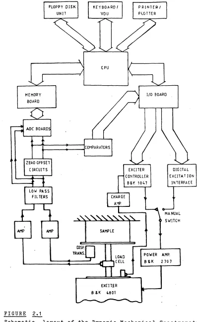
Figure 2.1 shows in schematic form the l ay ou t of the spectrometer. The system is based on c o m m e r c i a l l y a v a i l a b l e v i b r a t i o n e q u i p m e n t , i n c l u d i n g an electromagnetic exciter (Bruel and Kjaer type 4801, with general purpose head) and associated power amplifier (B &
K type 2707) and exciter control (B & K type 1047)* This equipment is designed for operation above 2 Hz, although
FLOPPY D I S K KEYBOARD f P R I N T E R /
UNIT VOU PLOTTER
1/0 EOARu MEMORY
BOARD
ADC BOARDS
COMPARATORS
ZERO OFFSET
CIRCUITS DIGITAL
EXCITAT ION
i n t e r f a C e
EXCITER CONTROLLER
B&K 10AT LOW PASS
FILTERS CHARGE
MANUAL SWITCH
SAMPLE
D1SP. TRANS
■ ■ • LUAU
IT xw
POWER AMP.B t K 2 7 0 7 EXCITER [image:27.619.85.482.26.672.2]B & K 4801
FIGURE 2.1
both the exciter and power amplifier will work at reduced specifications down to dc [3,4,5]. For operation at very-low f re q ue n ci e s a d i gi t al sine w av e is produ ce d by the microprocessor control system and output to the exciter via the d i g it a l e x ci t a t i o n interface. This inte rf ac e o p e r a t e s in the f r e q u e n c y r a n g e 0 . 0 6 - 1 8 Hz. F o r frequencies in the range 5-100 Hz the exciter control may be used to ge ne ra te the excit in g signal to the exciter
coils .
The c omputer c ontr ol system is based on a N as c o m III
d ed icated mi cr oc o mp ut e r, m a n u f a c t u r e d by Lucas Logic. The c o m p u t e r ha s d is c s t o r a g e f a c i l i t i e s an d is
i n terfac ed to an 80 c o l u m n dot matrix pri nt er (Epsom RX 80) and a W a t a na be p e r s o n a l p l o t t e r (WX4636). The Nascom III contains several operating systems including a P a s c a l l a n g u a g e c o m p i l e r a n d a c o m p r e h e n s i v e
e d i t o r / a s s e m b l e r , both of w hic h are disc loaded. The Nas co m III uses the v e r s a t i l e Z80A Cent ra l p r o c e s s i n g
unit and a total of 48K bytes of dynamic r an d om access memory (RAM) are available. The system clock is 4 MHz.
In order to specify the dynamic mechanical properties of the test piece, two input s i g n a l s are required. These
are the dynamic d e f o r m a t i o n of the test piece, and the force required to produce this deformation. The control s y s t e m m e a s u r e s the f r e q u e n c y of o p e r a t i o n , the amplitudes of the force and deformation signals and their
highly non-linear the mechanical properties will only be
meaningful if they are measured at a constant deformation a m p l i t u d e t h r o u g h o u t the f r e q u e n c y ra ng e. The s p e c t r o m e t e r p r o v i d e s f a c i l i t i e s for c o m p r e s s i n g the s i g n a l s to c o n s t a n t d i s p l a c e m e n t a m p l i t u d e . The amplitude of the dynamic oscillation may be set anywhere in the range 0.01-8 mm, subject to the limitations of the electromagnetic exciter.
The s o f t w a r e c o n t r o l s y s t e m a l l o w s the a u t o m a t i c
m e a s u r e m e n t of the dynamic storage m o d u l u s and loss tangent throughout the frequency range. Data acquisition
and a n a l y s i s are f u l l y automatic. The r e s u l t s can be stored on floppy disc for future analysis or printout. A special feature of the spectrometer is the availability of au to ma tic mass compensation. For low s ti ffness test p i e c e s the i n e r t i a l f o r c e g e n e r a t e d by the m o v i n g
elements of the spectrome ter between the sample and the force transducer may mask the behaviour of the test piece at higher frequencies. The mass c o m p e n s a t i o n system
a l l o w s this c o n t r i b u t i o n to be r e m ov e d from the data. More d e ta i l s of the a l g o r i t h m used to a c h i e v e this are
given in section
2.4-Ap p en d ix I c ontains a sum ma ry of the s p e c i f i c a t i o n s of the d y n a m i c m e c h a n i c a l s p e c t r o m e t e r . M a n y of the co mp on en ts shown are c o m m e r c i a l l y a v a i l a b l e and the
relevant instruction manuals should be consulted for the
Kjaer eq ui pm ent [3,4,5] and the tr an sd uc er s [9,10,11]• With the exception of the transducers, only the equipment
which has teen specially constructed or modified for the present application will he discussed.
2.3 The Electrical Hardware
2.3*1 Digital Excitation Output Interface
This i nt erfac e e na b l e s the m i c r o c o m p u t e r to produce a digital sine wave, with variable frequency and amplitude,
to d r ive the exciter at low frequencies. The sine w a v e is maintained in memory as a series of 1000 discrete data points which are output to the interfac e at r e g u l a r
intervals using a counter timer circuit, which produces a CPU interrupt after a programmed time interval. The rate at which the i n d i v i d u a l points are sent d e t e r m i n e s the frequency of the resulting signal. The data is delivered to a 12-bit d igital to a n a l o g u e c o n v e r t e r (DAC) via two parallel input/output (PIO) ports and results in a sine
w a v e of fixed a mp litude. A further DAC (8-bit) is required to specify the amplitude.
Figure 2.2 shows the c i r c u i t r y used for the d i g it a l e x c i t a ti on interface. A s in g l e data byte is output to
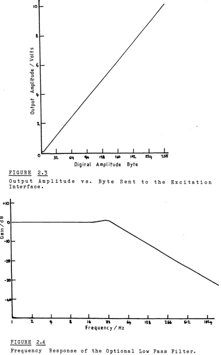
the 8-bit DAC (IC 1) to form a v o l t a g e p r o p o r t i o n a l to the required amplitude. This is a m p l i f i e d by IC 2 to produce a dc v o l t a g e in the range 0-10 Volts. This v o l t a g e forms the r ef er en ce to the 12-bit DAC (IC 3).
Figure 2.3 shows the variation of this reference voltage
^MOLS
^0 3 oocO
«m
■U O
-P
C M
-pP ft
-P
P
o
CJ
o
•H
-P
co
•p
•H O
X
ft
ca
•p
•H
t*o •H
P
CO• I
CO I
ft
« p
cj
M
w i t h the a m p l i t u d e b y t e sen t f r o m the c o m p u t e r . Linearity is maintained down to very low levels (~1 00 mV) hut d i s t o r t i o n of the sine w a v e was foiind to occur if reference voltages lower than 150 mV are selected.
The sine w a v e data is fed into the 12-hit DAC and is converted into a voltage which is determined hy the hyte
sent and the reference voltage selected. IC 4 and IC 5 produce a bipolar output with a maximum amplitude of 10V.
In a d di t io n to the c i rc u i t r y shown in figure 2.2 each o p e r a t i o n a l a m p l i f i e r has its own r e c o m m e n d e d offset circuits [13]« The d i g it a l to a n a l o g c o n v e r t e r s in use are described more fully in the manufacturers data sheets
[
1 4,
1 5].
The r e s u l t i n g signal is not a true sine wave. In fact it is made up of a series of s m a l l hut disc re te steps. A fourier transform of the output signal shows a secondary
peak at a f r e qu e nc y d e t e r m in e d hy the n u mb e r of data points output per cycle. In the present s ys t em this s ec o nd a ry peak occurs at 1 kHz and is 50dB b e l o w the main signal. To reduce this f ur th er an o p ti o na l low pass
filter is included in the output stage of the interface. With a -3dB point at about 40Hz and an ultimate slope of
6dB per octave, this filter reduces the peak at 1 kHz by a further 27dB. Figure 2.4 i l l u s t r a t e s the f r e q u e n c y response of this filter circuit.
>
\ 6
Q .
<
O
^4 IU
Dig ital Amplitude Byte
FIGURE 2.3
O u t p u t A m p l i t u d e vs. B y t e S e n t to the E x c i t a t i o n Interface.
+10
cD
O
-30
TL Mi
F r e q u e n c y / H z
FIGURE 2.4
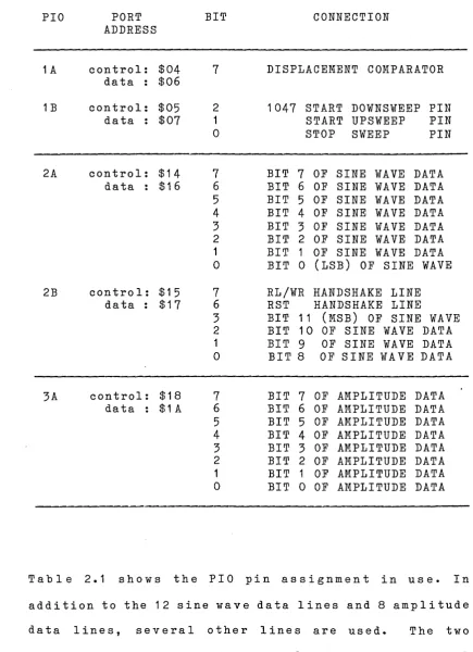
[image:33.614.65.509.15.727.2]TABLE 2.1 : PIO Pin assignment
PIO PORT
ADDRESS BIT CONNECTION
1 A control: $04 7 DISPLACEMENT COMPARATOR
data : $06
1 B control: $05 2 1047 START DOWNSWEEP PIN
data : $07 1 START UPSWEEP PIN
0 STOP SWEEP PIN
2A control: $14 7 BIT 7 OF SINE WAVE DATA
data : $16 6 BIT 6 OF SINE WAVE DATA
5 BIT 5 OF SINE WAVE DATA 4 BIT 4 OF SINE WAVE DATA 3 BIT 3 OF SINE WAVE DATA 2 BIT 2 OF SINE WAVE DATA 1 BIT 1 OF SINE WAVE DATA 0 BIT 0 (LSB) OF SINE WAVE
2B contro1: $15 7 RL/WR HANDSHAKE LINE
data : $17 6 RST HANDSHAKE LINE
3 BIT 11 (MSB) OF SINE WAVE 2 BIT 10 OF SINE WAVE DATA 1 BIT 9 OF SINE WAVE DATA 0 BIT 8 OF SINE W A V E DATA
3A control: $18 7 BIT 7 OF AMPLITUDE DATA
data : $1A 6 BIT 6 OF AMPLITUDE DATA
5 BIT 5 OF AMPLITUDE DATA
4 BIT 4 OF AMPLITUDE DATA
3 BIT 3 OF AMPLITUDE DATA
2 BIT 2 OF AMPLITUDE DATA
1 BIT 1 OF AMPLITUDE DATA
0 BIT 0 OF AMPLITUDE DATA
T a b l e 2.1 s h o w s the PIO pin a s s i g n m e n t in use. In a dd it io n to the 12 sine w a v e data lines and 8 a m p l i t u d e data lines, s e v e r a l other lines are used. The two h a nd sh ak e lines a ttached to bits 6 and 7 of PIO 2 port B are used to pass the sine wave data from the computer to
[image:34.616.62.498.89.690.2]For analogue signal generation using the exciter control unit, computer control is achieved using the three lines at ta ch ed to PIO 1 port B. These are c o n n ec t ed via t r a n s is to r in te rf a ce s to the rear panel of the exciter
control unit [5]* The three lines allow the frequency to be a l t e r e d by the c om p ut e r when the exci te r c on t ro l is used to provide the signal to the exciter coi'l s .
2.5*2 Memory Mapped Input ADC Interface
This i nt erfa ce p r o v i d e s a means of taking data into the
microprocessor. It is based around two type 1104 12-bit analogue to digital (ADC) boards, manufactured by Digital
D e si g n and D e v e l o p m e n t Ltd. Each board has a total of eight c h a n n e l s and software p r o g r a m m a b l e gains. Two
boards are used so that the d i s p l a c e m e n t and force s i g na l s can be s a m p l e d at the same time. Six of the eight channels on each board are unused.
The boards h av e been m em or y m ap pe d into the N a s c o m III. Memory mapping is a technique by which the board appears, to the c en tr al p r oc e s s i n g unit (CPU), to act as a b l o c k of memory. The CPU can write to and read from the boards
using n or m al m e mo ry i n t e r r o g a t i o n ins tructions. This r e su l ts in the time requi re d to enter data into the computer being reduced, and simplifies the software.
data is sent to the CPU in the form of two bytes), there are s e v e r a l other lines to p r o v i d e a link betw ee n the
board and the CPU. The data lines may be connected
directly to the Nascom bus, the other lines require some
logic circuits. The input lines r equired by the 1104
boards are:
I/O SELECT - when LON the board is selected.
R/W - when HIGH the CPU may read data from the board. When LOW the board will accept data
written to it.
A0/A^ - these two lines d et er mi ne the addr es s on the board being w r it te n to or read from. 4
locations are required by each board.
The two boards are inserted into the c o m p u te r bus in p l ac e of one b l o c k of RAM. The CPU gene ra te s three bus lines which are of interest. These are C"S, 10) and WR.
In a dd it i on 16 address lines are present. T a b l e 2.2 shows the truth table for g e n e r a t i n g the lines R/W and a s in gle I/O SELECT from the CPU lines. The R/^ line may
be connect ed d i r e c t l y to the WR line from the CPU. The boolean algebra to determine I/O SELECT is given by
I/O SELECT = A + B.C = A.BTc” 2.1
where A, B and C are the three bus lines as shown in
table 2.2. Two I/O SELECT lines are required, one for each board. This is achieved by combining the I/O SELECT
from equation 2.1 with the address line A2» from the CPU. Table 2.3 shows the truth table for this. The two boards
I/O S e le c t
I/O S elect
[image:37.612.53.531.51.778.2]R/W
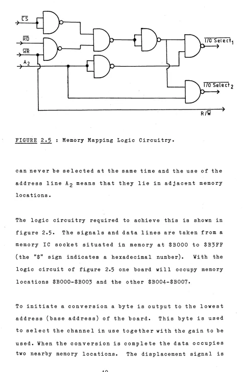
FIGURE 2.5 : Memory Mapping Logic Circuitry.
can n e v e r be s e l e c te d at the same time and the use of the address line A£ means that they lie in adjacent m emory locations.
The logic circuitry required to achieve this is shown in figure 2.5* The s ig na l s and data lines are taken from a memo ry IC socket situat ed in m e m or y at $B000 to $B3FF (the "$" sign indicates a hexadecimal number). With the
logic circuit of figure 2.5 one board will occupy memory
locations $B000-$B003 and the other $B004-$B007«
To i nitiate a c o n v e r s i o n a byte is output to the lowest address (base address) of the board. This byte is used to s el e ct the c h an n e l in use t o ge t he r with the gain to be
[image:37.612.44.519.62.384.2]TABLE 2.2 : Truth Table for the Handshake Logic
CPU A
SIGNALS
B C
BOARD REQUIRED
SIGNALS BOOLEAN ARITHMETIC FOR I/O SELECT
cs RD WR I/O" SELECT R/W
0 0 0 0 0 A
0 0 1 0 1 A
0 1 0 0 0 A
0 1 1 1 1 B AND C
1 0 0 1 0 A
1 0 1 1 1 A
1 1 0 1 0 A
1 1 1 1 1 A
TABLE 2.3 :Truth T able t 0 produce 2 I/O Select S i g n a 1 s
FROM TABLE
2.2 FROM THE CPU SIGNALS TO THE 1104 BOARDS
I/O SELECT A 2 I/O SELECT 1 I/O SELECT 2
0 0 1 0
0 1 0 1
1 0 1 1
1 1 1 1
connected to the lower board and the force signal enters the upper board.
2.3 »3 ■ Signal Conditioning Circuits
Three circuits assist in pas si ng each signal from the t r a n s du c er a m p l i f i e r s to the computer. The circuits e m p l o y e d for each of the input s ig n a l s are i d e n t i c a l in
a l l respects. The l o w - p as s f il t e r s and ze ro -o ff se t circuits p r o v i d e a means of i n c r e as in g the signal to
noise ratio and removing the unwanted dc component of the force and displacement signals. The comparator circuits, on the other hand, are used to p r o v i d e a t ri gg er for the microprocessor control system. This trigger informs the control system when to initiate measurements and enables the frequency to be measured. The frequency measurement is i n s e n s i t i v e to dc drift of the s i gn al s p r o v i d e d that the dc l e v e l c h a n g e s s l o w l y w i t h r e s p e c t to the
oscillatory signal.
Low-Pass Filters
These circuits provide a means of attenuating r.f. noise g en er at ed by n earb y equipment. They h av e a c ut - of f f r e q u e n c y of 500Hz. F i g u r e 2.6 s h o w s the c i r c u i t s i n v o l v e d . Becaus e an e x c e p t i o n a l l y flat r es po n se is required below the cut-off frequency a multi-stage active f i l te r circuit is used. Figure 2.7 shows the f r e q u e n c y characteristics of the filter. The ultimate slope of the f il t er s is > 3 0d B/o ct ave. The c ut-of f f r e q u e n c y is
o—
1 c
1 CFIGURE 2.6 : Low Pass Filter Circuit.
-l
i. I iiiiiu i i i m m
100
FREQUENCY/Hz
FIGURE 2 . 7 i Low Pass Filter Characteristics.
Zero-Offset Circuits
The control system incorporates an autoranging system to opti mi se the c o n v e r s i o n a cc ur a c y of the 1104 hoards. This s ys te m m ea su r es the a m p l i t u d e of the o s c i l l a t o r y signal and increases the gain as necessary. Any dc level on the s i g n a l s is no t t a k e n in to a c c o u n t hy the autoranging system and must he removed. Figure 2.8 shows
the circuit employed. A n e g a t i v e dc c om ponent is added
to the s i g n a l to o f f s e t the dc l e v e l f r o m the transducers. The offset voltage may he altered using the
cermet trimmer. F a c i l i t i e s for a ss i s t i n g with zeroing the s i gn a ls are p r o v i d e d in the c ontrol system. A residual dc component is permissahle, providing it does not exceed 20$ of the dynamic signal amplitude.
Comparators
A connection is taken from each input signal to PIO 1 of the c ompu te r via a comparator. Tah le 2.1 g i v e s the PIO pin assignment. The force signal c om p a r a t o r is present onl y for c om pl eteness. It is not used in the pres en t system. The circuit for each c o m p a ra to r is shown in figure 2.9- An operational amplifier is used in the open
loop mode. The output of this IC is either +15 or -15
Volts depending on the polarity of the input circuit with respect to the hias l e v e l , d et e r m i n e d hy the p o t e n t i a l divider. The transistor on the output reduces the signal to TTL levels. A light emiting diode on the output serves as an in di ca t or to show that the system is t r i g g e r i n g
fi s
tn
° V *
out
V:FIGURE 2.8 : The Zero-Offset Circuit.
CN
6-15
FIGURE 2.9 : The Comparator Circuit.
2.3*4 Transducers
Two t r a n s du ce r s are r equired to specify the m e c h a n i c a l p r o p e r t i e s of the te st p iece. T h e s e are a s e n s o r
m e a s u r i n g the d e f o r m a t i o n of the sample, and an i n- l i n e force transducer. A third transducer shown in figure 2.1 is an accelerometer which is used as part of the exciter control unit's compression loop [5]*
*
Force Transducer x
The load c e l l chosen for this a p p l i c a t i o n is a type U2,
strain gauge bridge c e l l ’ m a n u f a c t u r e d by H o t t i n g e r Baldwin Messtechnik GmBH. The conditioning amplifier is a MG 20, also m a n u f a c t u r e d by HBM. F u l l d e t a i l s of the transducer and amplifier are given in the manufacturers instruction manuals [9,10].
Strain gauge transducers proved best for this application
b ecause of their a b i l i t y to mea s ur e large loads at low frequencies, tolerate high side loads and are insensitive to dc drift. The transducer has a large mass (600g), but the provision of mass compensation facilities reduced the importance of this consideration. The chosen transducer has a f u l l scale m e a s u r i n g range of 2000 N in either
tension or compression.
Displacement Transducer
S e v e r a l tr an sd uc e rs were i n v e s t i g a t e d to meas ur e the d e f o r m a t i o n of t h e s a m p l e . T h e s e i n c l u d e d
a c c e l e r o m e t e r s p r o v e d u n s u i t a b l e b ecause the l e v e l of acceleration at low frequencies is too low. The LVDT is the commonest form of displacement measuring transducer.
They have the advantage of frictionless measurement and an essentially infinite resolution. They have several major disadvantages however for the present application. This includes difficulties in mounting on the sample, a
low frequency range and residual noise on the output.
A recent a d v a n c e in the m a n u f a c t u r e of IDMS sensors for the N u c l e a r power i nd u st ry has r e s u l t e d in p r o x i m i t y
d e te ct or s with large r m e a s u r i n g ranges [12]. These
transducers work by inducing high frequency eddy currents in a ferromagnetic target. This changes the impedence of
the o s c i l l a t o r circuit by an amount whi ch is d i r e c t l y related to the target-sensor gap. The transducer chosen for thi s a p p l i c a t i o n is the I - W - S 20 mm s y s t e m , m a n u f a c t u r e d by D o rn ie r GmBH. This type of t r a n s d u c e r has the a d v a n t a g e that it is n on-c on t ac t ing , is c a p a b l e of ope ra ti on up to high f r e qu en ci es and is i n h e r a n t l y noise free. In addition any non-conducting material may be p l a ce d b e tw ee n target and sensor with no effect on the measureme nt s. The system requires the p re se n c e of a
f e rr o ma g n e t i c target, a l t h o u g h it w i l l work ove r a smaller measuring range with targets such as aluminium or copper. More details of the I-W-S system may be found in the operating manual [11]•
2 • 4 The Measurement Algorithm
2.4.1 Theoretical Treatment
The system is r equired to meas ur e the a m p l i t u d e of the force and displacement signals and the phase difference
w i t h f r e q u e n c i e s in the r a n g e 0 . 0 7 - 1 0 0 Hz. It was necessary to devise a technique for determining the phase r e l a t i o n s h i p and the a m p l i t u d e s of each signal, which
w o u l d f u n c t i o n at v e r y l o w f r e q u e n c i e s an d w h i c h
minimised, the error due to noise. In this sec t io n the "basic mathematical method, its realisation as a numerical a l g o r i t h m and an a n a l y s i s of the effects of r an d om and harmonic noise are given. The signals of interest are of
the form:
where A, B-j and 6^ are time i n de p e n d e n t c on s ta n ts and T is the period of the waveform. The following half period integrals may he defined:
between them. These signals are essentialy sinusoidal
y ( t ) = A + B - | S i n [ 27Tt + 6.] ] 2.2
T
(i +2 )T/4
It = y ( t )at
. iT/4
i = 0,1,2,3 2.3
and it may he shown that
^1 = Iq " I2 = (2T Bj ) cos (<$ j ) TT
^2 = I? - 11 = (2TB1)sin(6 1) 2.4
The a m p l i t u d e and phase may be w r it te n in terms of ip ^
and i[>2 as
B1 = _L( Vf + '('I )1/2 2-5
2T
5 -| = tan” ^ ( ^ 2 / ^ 1 ) 2 ’^
Hence e v a l u a t i n g the four i n t e g r a l s in 2.3 a l l o w s the
direct d e t e r m i n a t i o n of B 1 and <51 and the r e s u lt is
i n d e p en d en t of the dc com po ne nt in the signal. The method has the advantage that it considerably reduces the effect of any random noise which has a c h a r a c t e r i s t i c time much less than T. H o w e v e r the method does depend upon the signal being m a i n l y s i n u s o i d a l and of known frequency. The errors i nt ro d uc ed by f a il u r e of these
assumptions are analysed in section 2.4 *3*
2.4*2 Numerical Methods
The input signals under consideration are taken into the computer in the form of N+1 points sampled at fixed time
intervals, tg , and covering one complete period. Figure 2.10 illustrates one input signal and defines many of the parameters to be used. The time period, T, of the signal has been measured previously and is given by
T = Nt + A T X s 2.7
t s t s
where - — < ATi £
-75-The four i n t e g r a l s are e v a l u a t e d for the force and