Phase relationships between two or more interacting processes from one dimensional time series II Application to heart rate variability data

Phase relationships between two or more interacting processes from one-dimensional

time series. II. Application to heart-rate-variability data

N. B. Janson,1A. G. Balanov,1 V. S. Anishchenko,2and P. V. E. McClintock1 1_{Department of Physics, Lancaster University, Lancaster, LA1 4YB, United Kingdom}

2_{Department of Physics, Saratov State University, Astrahanskaya 83, 410026, Saratov, Russia} 共Received 27 July 2001; published 15 February 2002兲

The recently proposed approach to detect synchronization from univariate data is applied to heart-rate-variability 共HRV兲 data from ten healthy humans. The approach involves introducing angles for return times map and studying their behavior. For filtered human HRV data, it is demonstrated that: 共i兲 in many of the subjects studied, interactions between different processes within the cardiovascular system can be considered as weak, and the angles can be well described by the derived model;共ii兲in some of the subjects the strengths of the interactions between the processes are sufficiently large that the angles map has a distinctive structure, which is not captured by our model; 共iii兲 synchronization between the processes involved can often be de-tected;共iv兲the instantaneous radii are rather disordered.

DOI: 10.1103/PhysRevE.65.036212 PACS number共s兲: 05.45.Xt, 05.45.Tp, 87.19.Hh

I. INTRODUCTION

A general approach has recently been proposed 关1,2兴for the detection of phase synchronization 共or its absence兲 be-tween two or more interacting processes based on the analy-sis of univariate data. The approach conanaly-sists in extracting return times from a continuous one-dimensional observable, reconstructing the return times map by delay embedding, and extracting phase angles. In the immediately preceding paper

关2兴, hereinafter referred to as Part I, we demonstrated ana-lytically and numerically that for two interacting processes these angles are in one-to-one correspondence with the con-ventional phase difference, and can thus be taken as an indi-cation of synchronization or otherwise. The same method was also extended to the case of several processes interacting in the presence of noise, and its workability was illustrated numerically for the case of three processes.

In the present paper we apply this approach to heart-rate-variability共HRV兲data from healthy human subjects in order to learn whether or not synchronization occurs for three of the most significant processes operating within the cardio-vascular system, namely, the main heart rhythm, respiration, and the process whose basic frequency is close to 0.1 Hz. The HRV data are in the form of R-R intervals extracted from electrocardiogrammes共ECGs兲.

II. DESCRIPTION OF DATA

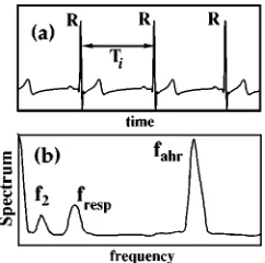
Figure 1共a兲shows a typical human ECG. The so-called R peaks, which are the largest ones, are indicated. The time intervals Ti between the two successive R peaks are usually called R-R intervals. They represent the time intervals be-tween the two consecutive heart beats and in terms of non-linear dynamics the time intervals between the trajectory’s return to a secant plane defined by the value of a threshold, i.e., return times. It is widely accepted that the human ECG has rather complex Fourier 共and wavelet兲spectra with well-distinguished characteristic peaks, three of them being espe-cially noticeable: a schematic Fourier power spectrum for a typical ECG is shown in Fig. 1共b兲. Usually these peaks are

associated with the rhythmic activity of certain physiological processes within cardiovascular system 共CVS兲: fahr defines the average heart rate; frespis associated with respiration pro-cess; the origin of f2⬃0.1 Hz is not quite clear at present—it is variously attributed to the sympathetic and parasympa-thetic nervous activity 关3兴, to the baroreflex loop关4兴, and to the intrinsic myogenic activity of the vascular smooth muscles 关5兴. At least two more distinguishable spectral peaks, at frequencies of about 0.01 and 0.03 Hz共not shown here兲, have recently been recognized 关5兴. However, on the small observation times with which we deal in the present research, they cannot be detected with confidence and, in the framework of this paper, we will treat them as additional manifestations of nonstationarity.

Qualitatively the same Fourier spectra can be obtained关6兴 from R-R intervals using a technique suggested in关7兴.

Thus, the dynamics of R-R intervals result from the com-plex interaction of several processes with different times-cales. With the exception of respiration and heart rate, there is usually 共but cf.关8兴兲 no possibility of gaining any knowl-edge about the phase or amplitude relationships between them with the use of noninvasive methods. It is, therefore, interesting to find out whether our technique can be helpful in order to detect the presence or absence of phase synchro-nization between the processes involved based solely on studies of the sequences of R-R intervals.

Data were recorded from 10 healthy students and young researchers of Saratov State University. Each ECG was reg-istered while the subject was resting in an armchair, over a period of 5–10 min, using a sampling rate of 180 Hz. For a test example of bivariate data, where both ECG and respira-tion signals were required, measurements were made at Lan-caster University during 3 min with a sampling rate of 400 Hz from a young healthy subject undergoing paced respira-tion with frequency of 0.5 Hz.

III. REMOVING THE FLOATING AVERAGE VALUE

As it was noted in Part I共Ref. 45兲 the return times of a nonstationary process usually oscillate around some ran-domly floating average value. In terms of the angles of return times map it means that the origin of this map is floating randomly. Angles extracted from such data are usually highly disordered and the useful phase information appears to be smeared. We are interested in the oscillations of return times around the average value, thus in order to gain ‘‘clean’’ phase information we advocate removal of this floating origin from return times prior to the extraction of angles. Any one of several existing methods can be used for this purpose, but here we discuss just two of them. We first show how they transform purely noisy data when no interactions take place

共Sec. III B兲, and then demonstrate their effect on a typical example of human HRV data共Sec. IV兲.

A. Description of filtering methods

In the present paper we use two different methods. The first of these consists of computing the analog of the second derivative of the original discrete time series x(i),

xder共i兲⫽

x共i⫹1兲⫹x共i⫺1兲⫺2x共i兲

2 . 共1兲

Let us refer to this method as to the method of derivatives. The second method is an extension of the well-known detrending technique. A local average is defined within a temporal window moving along the dataset which is then deduced from each datapoint. The only distinction of our method is that the size of the temporal window is not con-stant along the dataset. One window includes all points be-tween two successive extrema 共maximum and minimum, etc.兲of a discrete signal, including the extrema themselves. After the local average is computed within each window, its value is attributed to the time in the middle of the window. All such averages are then connected by straight lines by means of linear interpolation. Finally, from each original datapoint the value of the resultant graph is deduced 关see also Fig. 3共c兲兴. In what follows we will call this technique the method of differences.

Further, while plotting the filtered discrete data we will add them to the average value of the original unfiltered dataset.

B. Noisy oscillatory process without any interaction

Before attempting to apply our technique in practice to investigate interactions between oscillatory processes we

first need to know how the map of angles of return times behaves in the case when there are no deterministic interac-tions between processes being close to periodic, i.e., where only one noisy periodic oscillatory process occurs. Consider the Van der Pol oscillator in the presence of noise, i.e., Eq.

共2兲of Part I in the absence of external forcing (C⫽0), with noise intensity D⫽0.000 01,⑀⫽0.1, and␻⫽1. Let us record times tiwhen the phase trajectory intersects the level x⫽0 in one direction. The map for return times is presented in Fig. 2共a兲while the map for angles of return times in Fig. 2共b兲. It is easy to be convinced that the latter map contains no struc-ture by comparing it with those of Figs. 3 or 6 of Part I, representing Eqs. 共11兲or共19兲, respectively.

In order to check that the distinct structure that may ap-pear in map for angles is not merely due to the filtration procedures that we have used, we now apply the above filters to these purely noisy data. The results obtained after filtration are presented in Fig. 3共a兲 and 3共b兲. The presence of some structure in the resulting angles maps is quite obvious here— though it is far from being one dimensional, and neither is there any possibility of modeling these maps by means of Eq. 共19兲 in Part I. Note that the points concentrate in very specific regions, namely, between the return functions of Eq.

共11兲in Part I for␰⫽13 and␰⫽ 1

2 shown by gray dashed lines, and that they fill densely the interior and the vicinity of this FIG. 2. Van der Pol system forced only by Gaussian white noise of intensity D⫽10⫺5:共a兲return times map;共b兲angles map.

region. A typical feature of these maps is the existence of relatively sharp cusps pointing away from the diagonal. The origin of this structure can be explained phenomenologically using the basic property of white noise, namely, the nondif-ferentiability of its time series. That means that differences between the subsequent points change from negative to posi-tive very quickly. The probability of finding two successive local maxima 共or minima兲 being separated by only one or two points is much larger than the probability of finding a wider separation. An illustration of how the differences tech-nique works in this case is given in Fig. 3共c兲. In the upper plot the original dataset is shown together with the local average. After subtracting the latter one obtains a time series oscillating around zero with the current period varying ran-domly between 2 or 3. In terms of angles maps this means random 共and rapid兲 jumping between the return functions shown in Figs. 3共a兲and 3共b兲. Of course, due to total random-ness of the data, the whole map appears to be very noisy. The performance of derivatives technique can be explained in a similar way. Thus, if the shape of the angles map is similar to that presented in Fig. 3, we will consider these data as purely noisy.

IV. STAGES OF DATA PROCESSING

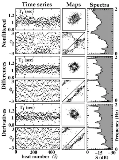
The stages in the processing of the measured R-R inter-vals are illustrated in Fig. 4.

An original sequence of R-R intervals is plotted 共Fig. 4, first row, first column兲. As usual, there is a slow variation of the average value, attributable to processes of very low fre-quency 共less than 0.1 Hz兲 which, over small observation times, can often be treated as nonstationarity. On the top

right is shown the Fourier power spectrum of the original HRV data 关6,7兴. The largest peak corresponds to the main heart rhythm fahr. Both this and the others of smaller ampli-tude are rather broad, presumably due to the nonstationarity. Correspondingly, the map of successive R-R intervals, being just the return times map共Fig. 4, first row, second column兲, usually has no distinct structure.

The angles ␾_i are extracted from the return times map

共Fig. 4, second row, first column兲, having placed the origin at the center of mass. A typical map for angles is as shown in Fig. 4 共second row, second column兲, where the points fall close to the diagonal near coordinate positions共␲/4;␲/4兲and

共⫺3␲/4; ⫺3␲/4兲 due to the predominance of very low-frequency oscillations influencing the heart rate 关compare with Fig. 6共a兲of Part I兴.

In order to concentrate on interactions of the main rhythm with respiration and the process with frequency⬃0.1 Hz, we need to reduce the effect of very low frequencies and subject the original sequence of R-R intervals to filtration. The re-sults of applying two filters described in Sec. III A usually differ slightly, and so in practice we compute the power spectrum for the each of the filtered data sets xder or xdiffin order to control the effect of filtering. In Fig. 4, rows three and four show the results of filtering by means of differ-ences, while rows five and six illustrate the workability of derivatives technique. The corresponding power spectra are shown at the end of each pair of rows. To compute the Fou-rier spectrum from filtered R-R intervals we just add to xder or xdiffthe average value of unfiltered R-R intervals, and then proceed in the same way as for original, nonfiltered data关6兴. The methods of differences and derivatives both remove the trend from the data, leading to return times maps共rows three and five兲 of similar appearance. However, the noisy back-ground of the power spectrum seems on average to be more uniform after filtration by derivatives, than by differences, although the use of derivatives leads to a more significant decrease of the lower-frequency range 共around 0.1 Hz and less兲. In both cases, two dominating frequencies and their combinations are clearly seen after filtration, but the ratios of their amplitudes appear to be slightly different. Note, that the derivatives technique is dangerous for data where the respi-ration frequency is less than a quarter of average heart rate. For such data we would recommend the use of differences as being the safer method.

The angles ␾i are extracted from the maps of filtered return times, and the map for angles共1兲from Part I is plotted

共Fig. 4, rows four and six兲. For the case considered, both angles maps seem to lie in the vicinity of the same curve being the return function of Eq.共11兲for in Part I␰⫽1

4 共 com-pare with Fig. 4兲. So both methods of filtration allow the structure of angles map in this example to be revealed more or less equally. Both of the ‘‘filtered’’ angles maps represent smeared continuous curves, and are definitely not formed by isolated clouds of points, thus testifying to the absence of synchronization between heart rate and the most dominant of the other processes 共which in the present case seems to be respiration兲. The rotation number ␰01 is estimated from Eq. 共21兲 of Part I to be

具␰典

具␰典

For further analysis of real data we select whichever filter leads to the more pronounced structure in the map for angles. Of course, neither of the filtration techniques described is perfect, and other techniques could be used instead to obtain similar or perhaps even better results.

Along with angles, the instantaneous radii were also ex-tracted from the human R-R intervals at each stage of pro-cessing. In Fig. 5 the maps for radii ri are shown for the same human data as in Fig. 4: for nonfiltered R-R intervals

共a兲, for those filtered by differences 共b兲 and by derivatives

共c兲. Unlike the angles␾i, the radii ri usually behaved in a rather disordered way, thus smearing the map of R-R inter-vals significantly. This remained true regardless of whether raw or filtered HRV data were used.

As shown in Part I, the map for angles of return times allows one to make a judgement about synchronization 共or its absence兲between the main rhythm and the other process with smaller amplitude, interaction with which is dominant. In the CVS the role of this second rhythm is usually played by respiration. The third rhythm often present in human HRV data has a basic frequency f2 that is close to 0.1 Hz and an amplitude comparable with or lower than that due to respi-ration. In order to obtain information about interaction be-tween respiration and the latter process, if it manifests itself in the power spectrum, we may finally proceed as suggested in Sec. III C of Part I, namely: extract the local maxima from the sequences of R-R intervals; filter the set of maxima by one or another technique; and then plot their map.

V. TESTING FILTERING ON SURROGATE DATA

Now, let us test filtering more thoroughly with the help of surrogate data关9兴. We are interested in the application of our method to data possessing the same Fourier power spectrum as real R-R intervals, but which is otherwise random. We obtained a set of surrogates for the dataset illustrated in Fig. 4 using the program surrogates from the TISEAN complex developed by the authors of this method关10兴, and then sub-jected it to all the same stages of processing. The results are presented in Fig. 6. Fourier spectra of either original or fil-tered surrogate data possess peaks at the same frequencies as the spectra of the reference data. They are of similar ampli-tude 共compare the spectra in Figs. 4 and 6兲, although not exactly the same, possibly due to the method of computing the spectrum used here 关7兴, which is not the fast Fourier transform used in 关10兴.

The angles maps look similar to those obtained for the purely random data of Figs. 3共a兲 and 3共b兲, and obviously

differ markedly from the corresponding maps derived from the reference data in Fig. 4.

VI. ANGLES OF RETURN TIMES MAP AND PHASE DIFFERENCE FOR HRV DATA

In Part I an explicit correspondence between the conven-tional phase difference and the angles of return times map was derived analytically and, what is of particular impor-tance for us here, confirmed for a simulated nonstationary process with floating eigenfrequency of oscillations. Here we attempt to establish the same correspondence for real bio-logical data. In order to evoke a regime of effective phase synchronization with the same rotation number ␰⫽1/3 as in the numerical simulation illustrated in Fig. 7 of Part I, we asked a healthy volunteer to breath at a frequency of 0.5 Hz, and measured both the ECG and respiration signals simulta-neously. The Fourier power spectrum of the HRV for this subject is given in Fig. 7, where the two main processes exhibit themselves through the presence of the peaks at fahr, f_resp, and their combinations 2 f_resp⫽f_ahr⫺f_resp. Thus, we FIG. 5. Map of radii of return times for the subject illustrated by

Fig. 12 for共a兲nonfiltered R-R intervals,共b兲R-R intervals filtered by

differences,共c兲R-R intervals filtered by derivatives.

FIG. 6. This figure illustrates the successive stages of processing of surrogate data for the dataset illustrated in Fig. 4 and compares the two filtering techniques. Details are discussed in the text.

can suppose that if any synchronization between heart rate and respiration takes place it has the order 1/3. We now proceed to analyze these data in exactly the same way as described in Sec. III A of Part I.

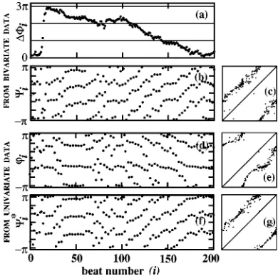
First, we undertake a conventional type of synchroniza-tion analysis, computing from the bivariate data the phase difference ⌬⌽i⫽␾ahr(ti)⫺3␾resp(ti) 关Fig. 8共a兲兴. The mo-ments ticorrespond to the appearance of R peaks in the ECG when its phase changes by 2␲, and the phase of respiration signal is taken as the phase angle of a phase portrait recon-structed by a suitable delay embedding from the respiration signal. We then construct the relative phase ⌿i and its map

关Figs. 8共b兲and 8共c兲, respectively兴. In Figs. 8共a兲and 8共b兲we can notice several horizontal segments testifying to the oc-currence of phase locking, and intervals where two phases slide against each other, i.e., are not locked.

Secondly, we perform the new type of synchronization analysis proposed in Part I, restricting ourselves to univariate data only. We choose for the latter the R-R intervals extracted from the ECG. We filter them by the derivatives method, extract angles ␾i and plot their map 关Figs. 8共d兲 and 8共e兲, respectively兴. Finally, we transform␾_i using Eq.共8兲of Part I to ‘‘reconstruct’’ the relative phase ⌿_i* whose temporal dependence and map are shown in Figs. 8共f兲 and 8共g兲, re-spectively关11兴.

The striking similarity between the plots in Figs. 8共b兲and 8共f兲, and 8共c兲and 8共g兲provides a convincing demonstration that the angles of a return times map are able to provide the same information as conventional phase difference and rela-tive phase. In other words, we have indeed been able to

extract essentially the same information about synchroniza-tion from the univariate time series as we obtained from two time series analyzed in the conventional way.

VII. SOME EXAMPLES OF EXPERIMENTAL ANGLE MAPS

In this section we present and discuss two examples of different phase and amplitude relationships between the three processes interacting within the CVSs of particular subjects. The first example is illustrated by Fig. 9. The R-R inter-vals are subjected to filtering by differences here, and the corresponding angles map in given in Fig. 9共a兲. The Fourier spectrum关Fig. 9共c兲兴reveals three distinct frequency compo-nents f_ahr, f_resp, and f₂, and the angles map共a兲is not close to any one-dimensional curve. Neither does it contain iso-lated clouds of points, so one can be confident that there is no phase locking between the main heart rhythm and respi-ration. Since there are three rhythms involved in the interac-tion, there are two independent rotation numbers, namely,␰01 for the interaction between heart beat and respiration, and␰12 for the interaction between respiration and the process with frequency f2. Formula 共21兲 of Part I, which is suitable for only two interacting processes, is not expected to provide a reliable estimate for any of the true ‘‘partial’’ rotation num-bers. However, the average rotation number

具

Now, consider the interaction between respiration and the process with f2. Extract local maxima from the original se-quence of R-R intervals, filter them by derivatives; extract angles, and create their map 关Fig. 9共b兲兴. A one-dimensional structure is quite evident here, although it cannot be de-scribed by Eq.共11兲in Part I共cf. the plots in Fig. 3 of Part I兲. The probable reason is that the amplitude of the process with f2is not much less than that of respiration, but is comparable with it. Thus approximation of Eq.共11兲in Part I is no longer valid, and we have no right to apply formula共21兲of Part I to estimate the rotation number. The observed map contains no isolated groups of points and can be taken as evidence for the absence of phase locking between respiration and f2. Thus, in the example considered no two of the three processes in-volved are synchronized with each other.

FIG. 8. Comparison of different methods used for the detection of phase synchronization in the human cardiovascular system. The first two rows of plots were derived from bivariate data共ECG and respiration兲: 共a兲 the conventional phase difference ⌬⌽i between respiration and ECG; 共b兲 relative phase ⌿i; 共c兲 map of relative phase⌿i⫹1vs⌿i. The third and fourth rows were obtained from

univariate data:共d兲angles of map of R-R intervals with removed floating average value;共e兲map of angles;共f兲angles transformed by means of 共8兲of Ref.关1兴;共g兲 map of transformed angles. Note the striking similarity between plots共b兲and共f兲, and共c兲and共g兲, respec-tively.

FIG. 9. Example of a datafile where three time scales are im-portant, but no pair of them is synchronous.共a兲Map of angles of

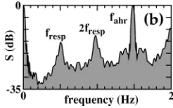
The second example is illustrated by Fig. 10. The power spectrum关Fig. 10共c兲兴contains distinguishable components of the main rhythm f_ahr and respiration f_resp, and much less pronounced combination frequencies fahr⫾f2. The first angles map 关Fig. 10共a兲兴 reveals a structure that is close to being one dimensional but which is not, however, captured by model共11兲in Part I 共compare with plots in Fig. 3兲. The reason is that, as in case of Fig. 10共b兲, interaction between the main process and respiration cannot be treated as weak; the latter conclusion is supported by the presence at rela-tively large amplitude of second harmonics of the respiration frequency 2 fresp and also the combination frequency ( fahr

⫺2 fresp). In this case too we cannot estimate the rotation number␰01by means of Eq.共21兲of Part I. However, in spite of the rather strong interaction, no synchronization between the basic process and respiration can be detected, since the angles map is close to a continuous curve. We now eliminate the main rhythm by selecting local maxima of R-R intervals, filter them by derivatives, and plot the corresponding map for angles 关Fig. 10共b兲兴. It clearly contains several isolated clouds of points, whose exact number will be discussed be-low: they constitute evidence of phase locking between the processes considered. The average rotation number ␰12 can be estimated as

具␰典

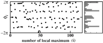
Since the numerator of the rotation number, if synchroni-zation exists, seems to be n⫽2, let us apply the technique used in Ref. 关12兴 to detect phase locking. Namely, unwrap the angles allowing them to increase monotonically, and then wrap them into an interval关⫺2␲; 2␲兴that is twice as large as 关⫺␲; ␲兴 关Fig. 11共a兲兴. Now, compute the probability den-sity for this dependence关Fig. 11共b兲兴. We find that it posseses 5 distinct peaks. This allows us to infer the existence of 2/5 synchronization between respiration and the process with f2, at least in the statistical sense关12兴.

VIII. MODELING ANGLES OF R-R INTERVALS

Let us apply the theoretical map共19兲of Part I to simulate the observed angles maps. For simplicity we set all phase

shifts ␾0_j to zero. First, we simulate the map of Fig. 8共e兲by setting frequencies ␻0⫽1, ⍀1⫽1/3, ⍀2⫽0.1; amplitudes A1⫽0.1, A2⫽0.01; the intensity of Gaussian white noise modulating the value of⍀1 as D⫽0.00002, the noise added to the right-hand part of model map D⫽0.06, and also some ‘‘measurement noise’’ added to the solution with intensity D⫽0.05. Since the number of points in Fig. 8 is about 200, for a good comparison the same number of points of the map

共19兲in Part I with the given parameter values are presented in Fig. 12共a兲. The two phase portraits are evidently very similar.

Secondly, we simulate the case of Fig. 10共b兲 by setting: frequencies ␻0⫽1, ⍀1⫽0.4, ⍀2⫽0.112... 共a long random sequence of numbers from 1 to 9兲; amplitudes A1⫽0.2, A2

⫽0.05; and the intensity of Gaussian white noise added to the equation D⫽0.001. 100 points of the resulting phase portrait are given in Fig. 12共b兲: the result looks remarkably similar to that in Fig. 10共b兲. Note, that the rotation number

␰12 here is set to exactly 2/5, and the tendency to merge for the two clouds of points furthest to the right is clearly seen. This latter example serves as an argument supporting our inference of 2/5 phase locking between respiration and f2.

Thus, the derived general map 共18兲 from Part I 关and its particular case共19兲兴 allows the dynamics of real cardiovas-cular signals to be modeled, at least in those cases where the main process interacts sufficiently weakly with the others.

IX. DISCUSSION

The results presented in some sense contradict to the ear-lier conclusion 关13兴 that no distinct structure arises in the angles maps of human R-R intervals in the case of spontane-ous breathing, and can appear only for paced respiration at

FIG. 10. Example of a datafile where three time scales are im-portant. Respiration is not synchronous with heart rate, but is syn-chronous with the rhythm whose f2⫽0.1 Hz.共a兲Map of angles of R-R intervals. Note: the interaction between heart rate and

respira-tion is nonlinear, and so the map is not captured by Eqs. 共11兲or

共19兲in Part I.共b兲Map of angles extracted from the map of all local maxima of R-R intervals 共note the distinct clouds of points兲. 共c兲 Fourier power spectrum关note the distinct second harmonic of res-piration frequency 2 frespand the combination ( fahr⫺2 fresp)兴.

FIG. 11. 共a兲Angles of the ‘‘secondary’’ return times map for a subject illustrated by Fig. 10, extended to the interval关⫺2␲; 2␲兴. The map of these angles is given in Fig. 10共b兲. 共b兲 Probability distribution of these angles, showing five peaks.

frequencies close to 0.1 Hz. We have demonstrated above that, although structure cannot be seen in the raw results, filtration of the data to remove the floating average value enables distinct structure to be observed for most healthy subjects. Thus, the deterministic structure revealed in angles map of filtered R-R intervals is the evidence of deterministic interaction between heart rate and, most probably, respiration and the oscillatory process at 0.1 Hz.

X. SUMMARY AND CONCLUSIONS

Based on the results presented above, we arrive at the following conclusions:

共1兲 In experimental heart-rate-variability data of healthy humans, the instantaneous radii ri are rather disordered, whereas the angles␾iof return times reveal much determin-ism in most of the cases considered.

共2兲The majority of the HRV data analyzed were success-fully modeled by the formulas共11兲and共19兲of Part I which was derived for the case of weak interaction. That means that interaction of the processes involved can be considered weak.

共3兲There are some data that contain distinct structure that is not captured by our models, thus revealing the existence of stronger interactions in some cases.

共4兲The technique presented allows one to study

synchro-nization between at least three processes interacting within the cardiovascular system.

The cardiovascular system is a particularly striking ex-ample of a system within which several oscillatory processes interact, mutually influencing each other. With the exception of respiration and the main cardiac rhythm, there is no pos-sibility of separating the signals from the individual pro-cesses in order to compare them and assess their synchroni-zation, or the lack of it, using conventional techniques. We have suggested and justified theoretically a tool 关1,2兴 to study interacting rhythms in the cardiovascular system using only heart rate variability data. We expect that the same ap-proach will be equally applicable to the other kinds of bio-medical signals with less or comparably complex structure. We hope that the proposed approach may prove to have po-tential for future applications and the development of new criteria for use in medical diagnostics.

ACKNOWLEDGMENTS

We are much indebted to Dr. Alexander Neiman for valu-able discussions and for his constructive comments on a draft version of the manuscript. The work was supported by the Engineering and Physical Sciences Research Council 共UK兲, the Leverhulme Trust, the Medical Research Council 共UK兲, and the U.S. Civilian Research Development Foundation

共Award No. REC 006兲.

关1兴N. B. Janson, A. G. Balanov, V. S. Anishchenko, and P. V. E. McClintock, Phys. Rev. Lett. 86, 1749共2001兲.

关2兴N. B. Janson, A. G. Balanov, V. S. Anishchenko, and P. V. E. McClintock, preceding paper, Phys. Rev. E 65, 036211

共2002兲.

关3兴S. Akselrod, D. Gordon, J. B. Madwed, N. C. Snidman, C. S. Shannon, and R. J. Cohen, Am. J. Physiol. 249, H867共1985兲; B. Pomeranz et al., ibid. 248, H151共1985兲.

关4兴B. W. Hyndman, R. I. Kitney, and McA. Sayers, Nature共 Lon-don兲233, 339共1971兲.

关5兴A. Stefanovska and M. Bracˇicˇ, Contemp. Phys. 40, 31共1999兲.

关6兴The Fourier spectrum of a sequence of interspike intervals was computed as suggested in Ref.关7兴. Namely, the signal to be processed was presented as a sum of ␦spikes placed at the time moments when R peaks occured in the electrocardio-gramme. The Fourier transform was then applied to the result-ant signal using its mathematical definition via an integral. This procedure allows one to pass from dimensionless

frequen-cies to real frequenfrequen-cies in hertz and to consider the full spec-trum, unrestricted by the usual 0.5/beat defined by the Nyquist theorem for discrete data.

关7兴R. W. DeBoer, J. M. Karemaker, and J. Strackee, IEEE Trans. Biomed. Eng. 31, 384共1984兲.

关8兴A. Stefanovska and M. Hozˇicˇ, Prog. Theor. Phys. Suppl. 139, 270共2000兲.

关9兴T. Schreiber and A. Schmitz, Physica A 142, 346共2000兲.

关10兴R. Hegger, H. Kantz, and T. Schreiber, Chaos 9, 413共1999兲.

关11兴As noted in Part I 关2兴, ⌿i* defines the relative phase up to some constant. While plotting Fig. 8共f兲we added to⌿i*a shift

0.3 chosen by trial in order to gain maximal similarity with Fig. 8共b兲.

关12兴C. Scha¨fer, M. G. Rosenblum, J. Kurths, and H.-H. Abel, Na-ture共London兲392, 239共1998兲.