and density-functional theories
T. J. P. Irons,1 J. W. Furness,1, 2 M. S. Ryley,1J. Zemen,1, 3 T. Helgaker,4and Andrew M. Teale1, 4,a)
1)
School of Chemistry, University of Nottingham, University Park, Nottingham, NG7 2RD, UK
2)Department of Physics and Engineering Physics, Tulane University, New Orleans, LA 70118,
USA 3)
Institute of Physics, Academy of Sciences of the Czech Republic, Na Slovance 1999/2, CZ-182 21 Prague, Czech Republic
4)
Hylleraas Centre for Quantum Molecular Sciences, Department of Chemistry, University of Oslo, P.O. Box 1033 Blindern, N-0315 Oslo, Norway
(Dated: 18 October 2017)
A recently proposed variation principle [N. I. Gidopoulos, Phys. Rev. A 83, 040502(R) (2011)] for the de-termination of Kohn–Sham effective potentials is examined and extended to arbitrary electron-interaction strengths and to mixed states. Comparisons are drawn with Lieb’s convex-conjugate functional, which allows for the determination of a potential associated with a given electron density by maximization, yielding the Kohn–Sham potential for a non-interacting system. The mathematical structure of the two functionals is shown to be intrinsically related; the variation principle put forward by Gidopoulos may be expressed in terms of the Lieb functional. The equivalence between the information obtained from the two approaches is illustrated numerically by their implementation in a common framework.
PACS numbers: Valid PACS appear here
I. INTRODUCTION
Variation principles lie at the heart of many quantum-chemical theories, giving practical prescriptions for how to obtain the best electronic energy, wave function or electron density via optimization. They may also offer insight into the connections between traditionalab initio
wave-function based approaches and density-functional theory (DFT). In this work, we examine a new variation principle, proposed by Gidopoulos in Ref. 1 for the de-termination of the non-interacting system of relevance to Kohn–Sham theory.
The variation principle proposed by Gidopoulos con-sists of minimizing the left-hand side of the inequality
hΨ|Hˆ0(v)|Ψi −E0(v)≥0, (1)
with respect to variations of the potentialv, for a fixed electronic wave function Ψ corresponding to a system of interest—typically, the physical ground-state wave func-tion for the system. The energy E0(v) in Eq. (1) is the ground-state energy of a non-interacting system, asso-ciated with the non-interacting Hamiltonian ˆH0(v) =
ˆ
T+P
iv(ri), where ˆT is the kinetic energy operator. As
discussed in Ref. 1 the minimization of the left-hand side of Eq. (1) yields the Kohn–Sham non-interacting poten-tialvsassociated with a non-interacting system that has the same density as that of the chosen input wave func-tion Ψ. The same variafunc-tion principle was also described earlier by Davidson2 and used as a tool to understand
a)Electronic mail: [email protected]
the analytic properties of the first-order reduced density matrix associated with Ψ. This complements its use in Ref. 1, where it provides a tool for the optimization of the potentialv. Here we refer to Eq. (1) as theGidopoulos– Davidson variation principle.
At first glance, the Gidopoulos–Davidson variation principle appears to be markedly different from alterna-tive approaches for determining the Kohn–Sham system corresponding to a reference wave function or density. For example, in Levy’s constrained-search approach to DFT,3,4 a constraint on the electron density is explic-itly applied to determine the Kohn–Sham system. More closely related is the Lieb variation principle, which for a non-interacting system corresponds to maximizing the left-hand side of the inequality5
E0(v)−(v|ρ)≤Ts(ρ) (2)
with respect to variations of the potentialv for a given input electron densityρ. Here we introduce the notation (v|ρ) =R
v(r)ρ(r)dr. Both the Gidopoulos–Davidson and Lieb variation principles involve an unconstrained opti-mization overv, yielding the Kohn–Sham potentialvsas their optimizer. Furthermore, their functional derivatives are identical up to a sign.1,5
between the generalized functionals and the exchange– correlation energy DFT.
Having established the close connection between these alternative variation principles, we present some results from numerical implementation in a common framework in Section V, highlighting the equivalent information they yield both in the non-interacting limit and for arbi-trary interaction strengths. In Section VI, we make some concluding remarks and discuss possible directions for fu-ture work.
II. VARIATION PRINCIPLES
In this section, we review the Rayleigh–Ritz variation principles for pure and mixed electronic states and the Hohenberg–Kohn and Lieb variation principles of DFT.
A. Rayleigh–Ritz variation principle
Consider an electronic system described by a Hamilto-nian of the form
ˆ
Hλ(v) =−
1 2
X
i ∇2
i +
X
i
v(ri) +
X
i>j
wλ(|ri−rj|)
= ˆT+ ˆV + ˆWλ
(3)
where ˆT is the kinetic-energy operator, ˆV the external potential operator, and ˆWλ the electron–electron
repul-sion operator for a given electron–electron interaction strengthλ∈[0,1], such thatw0= 0 (for non-interacting systems) andw1= 1/|ri−rj|(for physical systems). At
a given interaction strengthλ, the ground-state energy of anN–electron eigenfunction Ψ of the HamiltonianHλ(v)
can be defined in the context of wave-function theory by varying the wave function Ψ according to theRayleigh– Ritz variation principle,
Eλ(v) = inf
Ψ∈WN
D Ψ
ˆ
Hλ(v)
Ψ
E
(4)
whereWN is the set of allL2-normalized, antisymmetric
N-electron wave functions with a finite kinetic energy,
WN =
n
ΨhΨ|Ψi= 1 ; PN
i=1h∇iΨ|∇iΨi<∞
o
. (5)
The Rayleigh–Ritz variation principle is well defined for all potentialsvbelonging to the vector spaceχ∗=L3/2+
L∞, which includes all Coulomb potentials.5
It is often more useful to work with mixed rather than pure states, giving thecanonical-ensemble Rayleigh–Ritz variation principle
Eλ(v) = inf
ˆ
γ∈KN
tr ˆγHˆλ(v) (6)
whereKN is the set all admissible ensemble density
ma-trices,
KN =
P
iλi|ΨiihΨi| |λi≥0,Piλi= 1,Ψi∈ WN .
(7)
Although the ground-state energy can always be defined as the greatest lower bound in either Eqs. (4) or (6), the formulation in terms of ensembles is more flexible, allowing for mixed-state solutions. This extra flexibil-ity is important to establish correspondence between the optimizers in the Rayleigh–Ritz variation principle com-monly used inab initio theory and the Hohenberg-Kohn variation principle used in DFT6.
B. Hohenberg–Kohn and Lieb variation principles
Being concave and continuous, the ground-state en-ergy defined in Eq.(4) may be expressed in terms of the
Hohenberg–Kohn variation principle
Eλ(v) = inf
ρ∈χ(Fλ(ρ) + (v|ρ)), (8)
where Lieb’s universal density functionalFλ is obtained
from the ground-state energy by theLieb variation prin-ciple:5
Fλ(ρ) = sup v∈χ∗
(Eλ(v)−(v|ρ)). (9)
The functionals Eλ and Fλ are a conjugate pair,
re-lated by mutual Legendre–Fenchel transforms. The vec-tor spaces of admissible densities and potentials are the Banach spacesχ=L3∩L1andχ∗=L3/2+L∞, respec-tively, encompassing allN-representable densities ρ∈χ
and all Coulomb potentialsv∈χ∗, with which the den-sity has a finite interaction energy.
The Lieb functional defined above is equivalent to the Levy–Lieb constrained-search functional when defined in terms of ensembles,
Fλ(ρ) = inf
ˆ
γ→ρtr ˆγ
ˆ
Hλ(0), (10)
where ˆHλ(0) = ˆT + ˆWλ. The relationship between the
functionals may be better understood by rewriting the Lieb variation principle of Eq. (9) in the form
Fλ(ρ) = sup v∈χ∗
inf ˆ
γ∈KN
tr ˆγHˆλ(v)−(v|ρ)
(11)
= sup
v∈χ∗ inf ˆ
γ∈KN
trˆγHˆλ(0)−(v|ρ−ργˆ)
, (12)
which may be viewed as minimization of trˆγHˆλ(0) with
respect to ˆγ subject to the constraint that ρˆγ −ρ = 0
with Lagrange multiplier v, corresponding precisely to the Levy–Lieb constrained-search functional in Eq. (10). We note that the Levy constrained-search functional for pure states
Fλ(ρ) = inf
Ψ→ρhΨ|
ˆ
Hλ(0)|Ψi (13)
is an upper bound to the Lieb functionalFλ(ρ)≥Fλ(ρ),
as Fλ in the Hohenberg–Kohn variation principle for all
potentialsv, the only difference being that the minimiz-ing densities withFλ are always pure states.
As shown in Ref. 6, there is a one-to-one correspon-dence between the ground-state densities obtained from the Hohenberg–Kohn variation principle with the Lieb functional as in Eq. (8) and from the Rayleigh–Ritz vari-ation principle with ensembles as in Eq. (6) but not with pure states as in Eq. (4).
III. GIDOPOULOS–DAVIDSON VARIATION PRINCIPLE
The variation principle of Gidopoulos in Ref. 1 allows for the determination of the non-interacting system of relevance to Kohn–Sham theory and may be written in the form
D0(Ψ) = inf
v∈χ∗
hΨ|Hˆ0(v)|Ψi −E0(v)
, (14)
where Ψ∈ WN is an electronic wave function
correspond-ing to the physical system of interest; typically the physi-cal ground-state wave function of ˆH1(v) for somev∈χ∗. The energyE0(v) is the ground-state energy of the non-interacting system, defined according to Eq. (4). Note thatD0(Ψ) is well defined sincehΨ|Hˆ0(v)|Ψi−E0(v)≥0 for each Ψ∈ WN by the Rayleigh–Ritz variation
princi-ple.
A. Relationship to Lieb variation principle
The Gidopoulos–Davidson variation principle is re-lated in a simple manner to the non-interacting Lieb vari-ation principle
F0(ρ) = sup
v∈χ∗(E0(v)−(v|ρ)). (15) To see the relation, we decompose the non-interacting expectation valuehΨ|Hˆ0(v)|Ψiin the manner
hΨ|Hˆ0(v)|Ψi=T(Ψ) + (v|ρΨ) (16)
where T(Ψ) = hΨ|Tˆ|Ψi and ρΨ are the kinetic energy and density yielded by Ψ, respectively. A comparison of the functionals in Eqs. (14) and (15) then gives
D0(Ψ) =T(Ψ)−F0(ρΨ) =T(Ψ)−F0(ρΨ), (17)
where we in the last step has replace the Lieb functional by the Levy constrained-search functional, noting that
ρΨ is pure-state representable. We conclude that that the Gidopoulos–Davidson functional of a given system is simply the total kinetic energy of this system minus the non-interacting Levy constrained-search functional.
Since the interacting Levy functional is the non-interacting Kohn–Sham kinetic energy,
F0(ρ) =Ts(ρ) (18)
we find that the Gidopoulos–Davidson functional is the Kohn–Sham kinetic-energy correlation energy,
D0(Ψ) =T(Ψ)−Ts(ρΨ), (19)
or alternatively
D0(Ψ) =hΨ|Tˆ|Ψi − inf Φ7→ρΨ
hΦ|Tˆ|Φi (20)
where Φ is a single Slater determinant describing the non-interacting Kohn–Sham system.
The relationship of the Gidopoulos–Davidson func-tional to the correlation kinetic energy is well known1. Here we see that, for pure states, the non-interacting Gidopoulos–Davidson and Lieb variation principles yield the same Kohn–Sham system from different directions. The Lieb variation principle minimizes the value of the non-interacting kinetic energy Ts, subject to a den-sity constraint, whilst the Gidopoulos-Davidson varia-tion principle maximizes the correlavaria-tion kinetic energy
Tc=T−Ts subject to a similar density constraint. Fol-lowing the discussion in Section II B, we observe that that potential in Gidopoulos–Davidson variation principle in Eq. (14) may be viewed as the Lagrange multiplier for density constraint in Eq. (20).
B. Objective functions
Being related in such a simple manner, the optimiza-tions of the Gidopoulos–Davidson and Lieb functional are also related in a simple way. Expressing the functionals in terms of their objective functions, we find
D0(Ψ) = inf
v∈χ∗G0(v,Ψ) (21)
F0(ρ) = sup
v∈χ∗
L0(v, ρ) (22)
where
G0(v,Ψ) =hΨ|Hˆ0(v)|Ψi −E0(v) (23)
L0(v, ρ) =E0(v)−(v|ρ). (24)
Hence, we obtain in agreement with Eq. (17),
G0(v,Ψ) =T(Ψ)−L0(v, ρΨ). (25)
The functional L0(v, ρ) is concave in v and affine in ρ, whereasG0(v,Ψ) is convex in v. After a generalization to mixed states,G0 becomes convex also in the second variable; see Section III D.
C. Functional derivatives of objective functions
unique densityρv. For a given Ψ∈ WN, the expectation
value hΨ|Hˆ0(v)|Ψi is always differentiable with respect tov, with functional derivativeρΨ. Hence, assuming dif-ferentiability ofE0 atv, we have
δG0(v,Ψ)
δv(r) =ρΨ(r)−ρv(r), (26)
and7
δL0(v, ρ)
δv(r) =ρv(r)−ρ(r). (27)
When ρ = ρΨ, the functional derivatives are identical except for the sign difference.
The second derivatives of G0 and L0 with respect to the potentialv may also be readily evaluated. They are equal to (minus and plus) one half the non-interacting static density response function of the system7,
δ2G0(v,Ψ)
δv(r)δv(r0) =−
δ2L0(v, ρ)
δv(r)δv(r0) =− 1 2χ0(r,r
0)
=−1
2 X
ia
ϕi(r)ϕ∗i(r0)ϕa(r0)ϕ∗a(r)
εi−εa
+ c.c.,
(28)
where the indicesiandadenote occupied and virtual or-bitals, respectively, whose orbital energies areεi andεa.
In Ref. 1 focus is placed on the optimization ofG0 with respect tov. In passing, we note that the non-interacting Hamiltonian readily separates into one-electron contribu-tions ˆH0(v) =Pkˆhk(v) with ˆhk(v) =−12∇2k+v(rk) and
that the orbitals entering Eq. (28) are the eigenfunctions of this one-electron Hamiltonian. The non-interacting ground-state energy is the sum of the occupied orbital energies,E0(v) =Piεi. We also remark that, although ±1
2χ0(r,r
0) is positive/negative semi-definite, this does
not imply thatG0/L0 are convex/concave invsince the derivatives in Eq. (28) are not defined for all potentials. Throughout this discussion we have assumed the dif-ferentiability of L0(v, ρ) and G0(v,Ψ). The functional
L0(v, ρ) is not straightforwardly differentiable as dis-cussed by Lammert8, however this issue can be avoided by using a regularized form as discussed in Ref. 9. Since the derivative ofG0(v,Ψ) amounts to taking the deriva-tive of−L0(v, ρΨ) (see Eq. (25)), the same regularization techniques can be applied to this functional.
D. Generalization to ensembles
Generalizing the Gidopoulos–Davidson functional for pure states Ψ∈ WN to canonical ensembles ˆγ∈ KN, we
obtain the functional
D0(ˆγ) = inf
v∈χ∗ tr ˆγ ˆ
H0(v)−E0(v)
.
=T(ˆγ)− sup
v∈χ∗ E0(v)−(v|ρΨ)
, (29)
where T(ˆγ) = tr ˆγTˆ. The ensemble Gidopoulos– Davdison functional is concave. To show concavity, we select ˆγ1,ˆγ2 ∈ KN and obtain for each 0 < ν < 1 the
inequality
D0(νγˆ1+ (1−ν)ˆγ2)
=νtr ˆγ1Tˆ+ (1−ν) tr ˆγ2Tˆ−F0(νρ1+ (1−ν)ρ2) ≤νtr ˆγ1Tˆ(1−ν) tr ˆγ2Tˆ−νF0(ρ1)−(1−ν)F0(ρ2) =νD0(ˆγ1) + (1−ν)D0(ˆγ2) (30)
where in the second step we have used the convexity of the Lieb functional.
Since Ψ occurs quadratically inD0(Ψ), a similar proof is precluded for the pure-state Gidopoulos–Davidson functional, which is indeed not concave. Note that, for pure states ˆγΨ =|ΨihΨ|, the ensemble Gidopoulos– Davidson functional reduces to the original functional:
D0(ˆγΨ) =D0(Ψ).
E. Generalization to arbitrary interaction strengths
The Gidopoulos–Davidson functional may be extended to interacting systems in the manner
Dλ(Ψ) = inf v∈χ∗
hΨ|Hˆλ(v)|Ψi −Eλ(v)
(31)
which is related to the Lieb functional via
Dλ(Ψ) =hΨ|Tˆ+ ˆWλ|Ψi −Fλ(ρΨ) (32)
and can re-expressed in the constrained-search form as
Dλ(Ψ) =hΨ|Tˆ+ ˆWλ|Ψi − inf
Φ7→ρΨ
hΦ|Tˆ+ ˆWλ|Φi. (33)
The first derivative of the objective functional,
Gλ(v,Ψ) =hΨ|Hˆλ(v)|Ψi −Eλ(v), is again a simple
den-sity difference,
δGλ(v,Ψ)
δv(r) =ρΨ(r)−ρv(r), (34)
and its second derivative can be expressed in terms of the
λ–interacting density response function
δ2G
λ(v,Ψ)
δv(r)δv(r0) =− 1 2χλ(r,r
0). (35)
To perform practical optimizations using Eq. (31), we therefore require knowledge not only of the kinetic energy associated with the input wave function Ψ but also the
λ-interacting two-electron interaction energy, Wλ(Ψ) = hΨ|Wˆλ|Ψi. In practice, these quantities can be computed
IV. ADIABATIC CONNECTION
The adiabatic connection considers the link between the non-interacting Kohn–Sham auxiliary and physically-interacting systems.10–13 In this approach, the interac-tion strength λ in Eq. (3) is varied between 0 and 1, whilst imposing the constraint that, at each interaction strength, the electron density ρλ remains fixed at that
of the physical system ρ1. Most frequently, a linear path between these two limits is considered,11where the Coulomb operator is simply scaled linearly by the value of λ. However, generalized ACs14 have been explored along non-linear paths.15,16In the present work, only the linear path is considered but the generalization to non-linear paths is straightforward.
For the Hamiltonian in Eq. (3), the λ–dependent universal density functional can be written in the constrained-search3–5 form for canonical ensembles,
Fλ(ρ) = min
ˆ
γ→ρtr ˆHλ(0)ˆγ (36)
where the minimization is over all density matrices ˆγ as-sociated with the input electron density ρ. This func-tional is convex in ρ, concave inλ and non-negative for
λ≥0. Theλ-interacting functional can be related to its non-interacting counterpart via
Fλ(ρ) =F0(ρ) +
Z λ
0
∂Fν(ρ)
∂ν dν, (37)
where the derivative is well-defined on the real axis as a right- or left-derivative. Evaluation of the derivative and application of the Hellmann–Feynman theorem17,18leads to an ab initio expression for the exchange–correlation energy
Exc(ρ) =
Z 1
0
Wλ(ρ)dλ. (38)
HereWλ(ρ) is the AC integrand
Wλ(ρ) = tr ˆγ ρ
λWˆ −EJ(ρ), (39) where ˆγλρis the minimizing ensemble state at interaction-strength λ. Furthermore, the exchange and correlation energies may be resolved into separate components, re-sulting in an expression for the correlation energy alone
Ec(ρ) =
Z 1
0
{Wλ(ρ)− W0(ρ)}dλ. (40)
For a review of the adiabatic connection, see Ref. 19. To make practical use of these expressions, approaches for the calculation of the λ-interacting wave functions yielding a chosen electron density are required; see, for example, Refs. 20–22. The constraint that the density is fixed for all λ may be easily enforced by supplying fixed argumentsρ and Ψ to Eqs. (9) and (31) for allλ. We now discuss our implementation of the (generalized) Gidopoulos–Davidson variation principle, exploring the close connections to the generalized Lieb functional nu-merically.
V. RESULTS
From the discussion in the Section III, it is evident that the Gidopoulos–Davidson and Lieb optimizations are suf-ficiently closely related that they may be implemented in a common computational framework. We first discuss some details of our implementation; we then demonstrate the equivalence of the two approaches by performing nu-merical optimizations for a set of small atomic and molec-ular systems.
A. Computational details
The variation principle given in Eq. (31) allows a value to be obtained for the generalized Gidopoulos–Davidson functional by evaluating its infimum with respect to v. If the density yielded by the reference wave functionρΨ isv–representable, the infimum becomes a minimum. To varyvsuch that an optimization over the potential may be carried out in a practical computational scheme, the potential is modelled using the basis-set expansion of Wu and Yang7,23
vλ(r) =vext(r) + (1−λ)vref(r) +
X
t
btgt(r). (41)
Herevext(r) is the external potential due to interaction of the electrons with the atomic nuclei,vref(r) is a fixed ref-erence potential chosen to ensure thatvλ(r) has the
cor-rect asymptotic behaviour, and{gt}are a set of Gaussian
basis functions with coefficients{bt}. The reference
po-tential employed in the present work is the Fermi–Amaldi potential24. With this choice of potential expansion, the derivatives corresponding to Eqs. (34) and (35) may be readily implemented as described in Refs. 7, 21, and 22, allowing the objective functional to be effectively opti-mized with respect to the set of coefficients{bt}.
An un-contracted form of the Gaussian basis set aug-cc-pVTZ25,26 in the spherical-harmonic basis is used for both the orbital expansion and for the potential expan-sion in Eq. (41), for all systems. An approximate Newton method is employed to accelerate convergence of the op-timization27, in which the Hessian is regularized using a truncated singular value decomposition with a threshold of 10−6 a.u. In all calculations, the convergence thresh-old was set to 10−6a.u. on theL2 norm of the objective functional gradient. To obtain a reasonably accurate ap-proximation to the Kohn–Sham system, the input quan-tities for each functionalFλ(ρΨ) and Dλ(Ψ) were
TABLE I. Optimized functional values and energy compo-nents calculated in the aug-cc-pVTZ basis using the variation principles of Eqs. (14) and (15). All quantities are in atomic units
F0 D0 Enn Ts Ene EJ Ex Ec T W E1
He 2.8611 0.0355 0.0000 2.8611 −6.7455 2.0464 −1.0232−0.0756 2.8967 0.9477 −2.9011 Be 14.5835 0.0661 0.0000 14.5835 −33.6945 7.2122 −2.6725−0.1534 14.6496 4.3863 −14.6586 Ne 128.5050 0.2720 0.0000 128.5050 −310.9007 65.9350−12.0691−0.6071 128.7765 53.2589−128.8654 H2(R= 0.7) 1.7263 0.0324 1.4286 1.7263 −4.8614 1.6508 −0.8254−0.0700 1.7588 0.7554 −0.9187 H2(R= 1.4) 1.1390 0.0328 0.7143 1.1390 −3.6469 1.3215 −0.6607−0.0729 1.1718 0.5879 −1.1729 H2(R= 3.0) 0.8279 0.0418 0.3333 0.8279 −2.6181 0.9539 −0.4769−0.1184 0.8697 0.3586 −1.0564 H2(R= 5.0) 0.9520 0.0224 0.2000 0.9520 −2.3809 0.8193 −0.4097−0.2063 0.9744 0.2033 −1.0033 H2(R= 7.0) 0.9919 0.0052 0.1429 0.9918 −2.2826 0.7669 −0.3835−0.2406 0.9971 0.1429 −0.9998 H2(R= 10.0) 0.9981 0.0005 0.1000 0.9982 −2.1983 0.7245 −0.3623−0.2623 0.9986 0.1000 −0.9997
B. Kohn–Sham non-interacting system
In Table I, the optimized values of the non-interacting Lieb functional F0(ρΨ) and Gidopoulos–Davidson func-tional D0(Ψ) are presented for a series closed–shell atoms and for the hydrogen molecule at several bond lengths. Additionally, Kohn–Sham energy components are presented, including the internuclear repulsion energy
Enn, the non-interacting kinetic energyTs, the electron– nuclear attraction Ene, the Coulomb energyEJ, the ex-change energyEx, and the correlation energyEc. These components have the same definition when computed from F0(ρΨ) and D0(Ψ). For comparison, the total ki-netic energyT and total electron–electron interaction en-ergy W are included, along with the total interacting ground-state energyE1.
The consistency of the optimizations was verified by comparing the optimized values of F0(ρΨ) and D0(Ψ) presented in Table I with the energetic components Ts andTcrespectively. The value ofTswas determined from the Kohn–Sham orbitals obtained atλ= 0 and the value ofTcwas obtained by subtraction ofTsfromT, where the latter was determined directly from theλ= 1 calculation. The H2molecule provides a simple prototypical system with which the variation between dynamic and static cor-relation may be explored. At equilibrium geometry, the electron densities of the two hydrogen atoms overlap sub-stantially, thus binding the molecule and leading to both kinetic and potential contributions to the correlation en-ergy. As the interatomic bond is extended, the system approaches that of two isolated hydrogen atoms, with no kinetic correlation energy; see Table I, where the value of the Gidopoulos–Davidson functional D0 decreases as the interatomic bond length R increases, becoming just 0.0005 a.u. atR= 10.0 a.u.
C. General interaction strengths
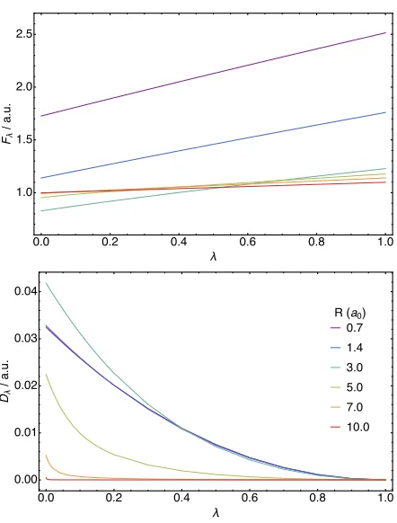
In Figure 1, results of optimizations pertaining to the generalized Lieb and Gidopoulos–Davidson functionals, according to Eq. (9) and Eq. (31), respectively, are pre-sented for interaction strength λin the range 0 to 1. In the upper panel, the Lieb functionalFλ(ρΨ) is shown as a function of λ for the H2 molecule with bond length
R = 0.7, 1.4, 3.0, 5.0, 7.0 and 10.0 a.u. The varia-tion of Fλ(ρΨ) in λ is broadly linear, indicating that
��� ��� ��� ��� ��� ���
��� ��� ��� ���
λ �λ
/
����
�(��)
��� ���
��� ���
��� ����
��� ��� ��� ��� ��� ���
���� ���� ���� ���� ����
λ
�λ
/
����
FIG. 1.Fλof Eq. (9), upper panel, andDλof Eq. (31), lower panel (a.u.) as functions of the interaction strengthλfor the H2molecule at internuclear separationsR= 0.7, 1.4, 3.0, 5.0, 7.0 and 10.0 a.u.
Tc,λ=T1−Tλis relatively small and reflecting the
domi-nance of the Coulomb and exchange energies in the two– electron energy W, both of which are linear in λ. The slope ofFλ(ρΨ) inλbecomes progressively smaller as the bond length is increased. This behaviour reflects the fact that the H2 molecule dissociates into two one-electron fragments withλEJ+λEx+Ec,λ→0 asR→ ∞(static
correlation energy cancelling the Coulomb and exchange energy).
In the lower panel of Figure 1, the Gidopoulos– Davidson functionalDλ=T1−Tλ+λ(W1−Wλ) is also
D. Constructing the adiabatic connection
As described in subsection IV, the AC comprises a link between the non-interacting Kohn–Sham auxiliary system and the physically interacting system through variation in interaction strength, modulated by coupling– constant λ, with the density equal to the physical den-sity ofλ= 1 for allλ. The AC integrand is expressed in Eq. (39), from which an exact definition of the correlation energy may be constructed according to Eq. (40). Given that the exchange energy scales linearly withλ (for the linear–attenuation AC path), the exchange contribution to Eq. (39) is simply a constant and may be subtracted to give the correlation component of the AC integrand,
Wc,λ(ρ) =Wλ(ρ)− W0(ρ). (42)
The Gidopoulos–Davidson variation principle of Eq. (31) and the Lieb variation principle of Eq. (9) can both be exploited to calculate this integrand, using the same in-putρΨ or Ψ but with a range of different values ofλ, to construct the AC using Eq. (42).
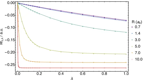
The equivalence of the AC curves constructed from the Lieb and Gidopoulos–Davidson functionals is con-firmed numerically for the H2 molecule at the same ge-ometries considered in Table I, with the AC integrands
Wc,λplotted as a function ofλin Figure 2. Here, values
of Wc,λ computed with the Lieb functional Eq. (9) are
represented by solid lines, whilst values obtained from the Gidopoulos–Davidson functional Eq. (31) are denoted by the point markers. It is evident from Figure 2 that the AC curves of these two methods agree to within the convergence of the optimization procedures.
The correlation energy can be computed from these curves using Eq. (40) and the numerical values ofEc are presented in Table I. The ratio |Ec|/Tc has been used to assess the relative importance of static correlation31. The |Ec| corresponds to the area above each curve in Figure 2, whilstTc corresponds to the area between each curve and a horizontal line defined by its value ofW1(Ψ). AsRincreases, this ratio grows and the curves approach an L shape characteristic of systems dominated by strong correlation, indicating that the value of Tc is approach-ing zero, consistent with the effects of hydrogen molecule dissociation discussed in subsection V C.
VI. CONCLUSIONS
The variation principle proposed in different con-texts by Gidopoulos1 and Davidson2 has been exam-ined and shown to be closely linked to the Lieb varia-tion principle.5 For the non-interacting system, the two functionals approach the Kohn–Sham system from differ-ent directions. The Lieb functional minimizes the non-interacting kinetic energy Ts subject to the constraint that the density is equal to that of the physical system, whereas the Gidopoulos–Davidson functional maximizes
[image:7.612.318.561.51.187.2]●●●●●●●● ● ● ● ● ●● ● ● ● ● ● ● ● ● ● ● ● ■ ■ ■■■■■ ■ ■ ■ ■ ■■ ■ ■ ■ ■ ■ ■ ■ ■ ■ ■ ■ ■ ◆ ◆◆◆◆◆◆◆◆ ◆◆ ◆◆◆ ◆◆ ◆ ◆ ◆ ◆ ◆ ◆ ◆ ◆ ◆ ▲ ▲ ▲▲ ▲▲ ▲ ▲ ▲ ▲ ▲ ▲ ▲ ▲ ▲ ▲ ▲ ▲ ▲ ▲ ▲ ▲ ▲ ▲ ▲ ▼ ▼ ▼ ▼ ▼ ▼ ▼ ▼ ▼ ▼ ▼ ▼ ▼▼ ▼ ▼ ▼ ▼ ▼ ▼ ▼ ▼ ▼ ▼ ▼ ○ ○ ○ ○ ○ ○ ○○ ○ ○ ○ ○ ○ ○ ○ ○ ○ ○ ○ ○ ○ ○ ○ ○ ○ ��� ��� ��� ��� ��� ��� -���� -���� -���� -���� -���� ���� λ �� � λ / ���� �(��) ● ��� ■ ��� ◆ ��� ▲ ��� ▼ ��� ○ ����
FIG. 2. The correlation adiabatic connection integrand values (a.u.) of Eq. (42), calculated using the optimization of Eq. (9), lines, and Eq. (31), point markers, for the H2 molecule at internuclear separationsR = 0.7, 1.4, 3.0, 5.0, 7.0 and 10.0 a.u.
the kinetic correlation energyTcunder the same density constraint. In both cases, an unconstrained optimization can be performed with respect to the potential expan-sion coefficients in Eq. (41), making the implementation straightforward as described in Refs. 7 and 21. The ex-ternal potential plays the role of a Lagrange multiplier function, which ensures that the density constraint is sat-isfied at the stationary point for each functional.
An extension of the Gidopoulos–Davidson functional to ensembles was also presented, for which the associ-ated functional can be shown to be concave with respect to ˆγ. This contrasts the pure-state functional which is not concave with respect to Ψ. A further extension to treat general electronic interaction strengthsλ was also presented, as has previously been done with the Lieb functional.5,7,20–22 Utilizing this extension, it was shown that either functional may be used to calculate the adia-batic connection between the Kohn–Sham system of non-interacting electrons and the physically-non-interacting sys-tem, highlighting the fact that the two functionals are essentially equivalent, being related simply by a constant
T(Ψ) and a change of sign. As such, they are amenable to implementation in a common computational framework.
ACKNOWLEDGEMENTS
Research Council (EPSRC), Grant No. EP/M029131/1, and the Nottingham High Performance computing ser-vice. A. M. T. gratefully acknowledges support from the Royal Society University Research Fellowship scheme.
1N. I. Gidopoulos,Phys. Rev. A83, 040502 (2011).
2E. R. Davidson, Reduced Density Matrices in Quantum
Chem-istry, volume 6 ofTheoretical Chemistry, Elsevier BV, 1976.
3M. Levy, Proceedings of the National Academy of Sciences76,
6062 (1979).
4M. Levy and J. P. Perdew, Int. J. Quantum Chem. 21, 511
(1982).
5E. H. Lieb, Int. J. Quantum Chem.24, 243 (1983).
6S. Kvaal and T. Helgaker,J. Chem. Phys.143, 1184106 (2015). 7Q. Wu and W. Yang, J. Chem. Phys.118, 2498 (2003). 8P. E. Lammert, International Journal of Quantum Chemistry
107, 1943 (2007).
9S. Kvaal, U. Ekstr¨om, A. M. Teale, and T. Helgaker, J. Chem.
Phys.140, 18A518 (2014).
10D. Langreth and J. Perdew, Solid State Commun. 17, 1425
(1975).
11D. C. Langreth and J. P. Perdew,Phys. Rev. B15, 2884 (1977). 12O. Gunnarsson and B. I. Lundqvist, Phys. Rev. B 13, 4274
(1976).
13O. Gunnarsson and B. I. Lundqvist, Phys. Rev. B 15, 6006
(1977).
14W. Yang,J. Chem. Phys.109, 10107 (1998).
15J. Toulouse, F. Colonna, and A. Savin, Mol. Phys.103, 2725
(2005).
16A. M. Teale, S. Coriani, and T. Helgaker, J. Chem. Phys.133,
164112 (2010).
17H. Hellmann, Einf¨uhrung in die Quantenchemie, inHans
Hell-mann: Einf¨uhrung in die Quantenchemie, pp. 19–376, Springer
Science + Business Media, 2015.
18R. P. Feynman,Phys. Rev.56, 340 (1939).
19A. Savin, F. Colonna, and R. Pollet,Int. J. Quantum Chem.93,
166 (2003).
20F. Colonna and A. Savin, J. Chem. Phys.110, 2828 (1999). 21A. M. Teale, S. Coriani, and T. Helgaker, J. Chem. Phys.130,
104111 (2009).
22A. M. Teale, S. Coriani, and T. Helgaker, J. Chem. Phys.132,
164115 (2010).
23W. Yang and Q. Wu, Phys. Rev. Lett.89, 143002 (2002). 24E. Fermi and E. Amaldi, R. Accad. d’Italia. Memorie6, 119
(1934).
25T. H. Dunning,J. Chem. Phys.90, 1007 (1989).
26R. A. Kendall, T. H. Dunning, and R. J. Harrison, J. Chem.
Phys.96, 6796 (1992).
27Q. Wu and W. Yang, J. Theor. Comp. Chem.2, 627 (2003). 28QUEST, a rapid development platform for QUantum Electronic
Structure Techniques, 2017. http://quest.codes
29Numba, numba.pydata.org, 2017, Version 0.32.
30S. K. Lam, A. Pitrou, and S. Seibert, Numba, inProceedings of
the Second Workshop on the LLVM Compiler Infrastructure in HPC - LLVM’15, ACM Press, 2015.
31M. Ernzerhof, J. P. Perdew, and K. Burke, Int. J. Quantum