Munich Personal RePEc Archive
Exchange rate determination of
TL/US
:
aco
−
integrationapproach
Levent, Korap
Istanbul University Institute of Social Sciences, Besim Ömer Paşa
Cd. Kaptan-ı Derya Sk. 34452 Beyazıt /ISTANBUL
2008
Online at
https://mpra.ub.uni-muenchen.de/19659/
1
EXCHANGE RATE DETERMINATION OF TL/US$: A
CO-INTEGRATION APPROACH
Levent KORAP
*___________________________________________________________________________ Abstract
In our paper, we investigate exchange rate determination mechanism of TL/US$ for the 1987Q1-2006Q4 period using quarterly observations. Following a large literature review, we first highlight various approaches explaining monetary model exchange rate determination based on economic fundamentals, and then, construct an empirical model revealing both long-run stationary relationships and short-long-run dynamic adjustment processes of the nominal exchange rate for the Turkish economy. Our findings employing multivariate Johansen-Juselius type co-integrating approach indicate that nominal exchange rate is co-integrated with the fundamentals suggested by economics theory. Besides, short-run deviations from the fundamental-based equilibrium course of the nominal exchange rate have permanent effects on the long-run equilibrium exchange rate, and so have been stemmed from the existence of some form of hysteresis effects dominated in the nominal exchange rate.
Keywords: Exchange Rates; Sticky Price Monetary Model; Flexible Price Monetary;
Economic Fundamentals; Randow Walk; Co-integration; Hysteresis; Turkish Economy
Jel Classification F31; F41; F47.
___________________________________________________________________________
*Adres:
Economist, Marmara University Department of Economics
2
___________________________________________________________________________ Özet
Çalışmamızda, TL/US$ döviz kuru belirlenme mekanizması 1987Q1-2006Q4 döneminde üçer aylık veriler kullanılarak incelenmektedir. Geniş bir yazın taramasından yaralanılmak suretiyle öncelikle iktisadi temeller dahilinde oluşturulmuş döviz kuru belirlenme mekaniznasına yönelik çeşitli yaklaşımlar aydınlatılmış ve daha sonra parasal döviz kurunundan kaynaklanan hem uzun dönem durağan ilişkileri hem de kısa dönemli devinimsel uyum süreçlerini Türkiye ekonomisi koşullarında ortaya koyan uygulamalı bir model oluşturulmuştur. Çok değişkenli Johansen-Juselius eş-bütünleşim yaklaşımı kullanılarak elde ettiğimiz sonuçlar parasal döviz kurunun iktisat kuramı tarafından önerilen temeller ile eş -bütünleşik olduğunu göstermiştir. Ayrıca, parasal döviz kurunun iktisadi temeller dahilindeki denge yolundan kısa dönemli sapmaları uzun dönem denge döviz kuru üzerinde kalıcı etkiler göstermekte ve bu nedenle parasal döviz kuru içerisinde yerleşik bulunan histeresis türü etkilerin varlığı altında ortaya çıkmaktadır.
Anahtar Kelimeler: Döviz kurları; Katı Fiyat Parasal Modeli; Esnek Fiyat Parasal Modeli;
İktisadi Temeller; Rassal Yürüyüş; Eş-bütünleşim; Histeresis; Türkiye Ekonomisi
Jel Sınıflaması: F31; F41; F47.
___________________________________________________________________________
I. INTRODUCTION
3
Especially, for a small and open developing country such as Turkey, policy design process by the policy makers should be inclusive of the stylized facts based on these researches. Kesriyeli (1994), Metin (1994), Telatar and Kazdagli (1998), Bahmani-Oskooee and Kara (2000), Gokcan and Ozmen (2001), Dulger and Cin (2002), Civcir (2003a), Civcir (2003b), Civcir (2003c), Yazgan (2003), Erlat (2003), Ozdemir (2004) and a recent paper by Saatcioglu et al. (2007) give some empirical findings upon these issues of interest for the Turkish economy.
Of all these contemporaneous theoretical developments, a vast literature has been attributed to modeling the behavior of exchange rates so as to see whether monetary fundamentals are able to explain long-run course and short-run dynamics of exchange rates. What is of considerable interest in the economics literature is also to examine how well the out-of-sample forecasts fit with the actual data when assessing various estimation methods for forecasting purposes. Following the seminal paper by Meese and Rogoff (1983) indicating that fundamental based structural models of exchange rate do not beat the performance of the naïve random walk models in out-of-sample forecasts, there has been an extensive controversy upon these issues of interest. Researchers tend to explore whether the models based on structural relations or driven by naïve-random walks or considering more recent multivariate co-integration techniques, both assuming non-stationarity of data in the level form and preserving long-run knowledge of economic relations, must be of special interest, and to the extent that they produce more accurate estimates, models have been accepted to be superior when compared with the others.
4
monetary model but are also sensitive to the model specification as for the appropriate signs of the model in the sense that co-integrating vectors with plausible estimates are only obtained for Chile and Argentina but not for Israel. Likewise, Moosa (2000) examining the 1919-1923 German hyperinflation period gives evidence to the monetary model of exchange rate determination. Mark (1995) employing the US dollar prices of the Canadian dollar, the Deutsche mark, the Swiss franc and the Japanese yen finds that long-horizon changes in the logarithm of spot exchange rates are predictable. He gives evidence to that the out-of-sample point predictions from fundamental based models generally out-perform the driftless random walk model at the longer horizons. Kilian (1999) and Berkowitz and Giorgianni (2001) present a criticism to Mark’s (1995) methodoloy dealing with the data generating process used for predictability. Chinn and Meese (1995) support Mark’s conclusions to a great extent and find that fundamental-based error correction models out-perform the random walk model for long-term prediction horizons. Neely and Sarno (2002) give a brief summary of the seminal papers of Meese and Rogoff (1983) and Mark (1995) upon exchange rate determination mechanism considered in the economics literature.
MacDonald and Marsh (1997) also indicate that fully dynamic out-of-sample forecasts from simultaneous equations models incorporating meaningful long-run equilibrium and short-run dynamic relationships are cabaple of significantly out-performing those of a random walk model considering the US, Japan, UK and German data for the 1974-1990 period. Cheung and Chinn (1998) apply to a methodology using some consistency tests of evaluating exchange rate forecast rationality for Japanese yen, German Mark and Canadian dollar exchange rates against the US dollar for 1983-1993 and 1987-1993 periods, for which consistency requires that the forecast and the actual series (i) be the same order of integration, (ii) be cointegrated and (iii) yield co-integrating vector consistent with long-run unitary elasticity of expectations. They indicate that the first requirement generally holds, however co-integration fails to hold the longer the horizon. Of the co-integrating pairs, besides, the third requirement is not generally rejected.
5
fundamentals with respect to either the US dollar or Deutsche mark for the 1973-1994 period. However co-integration tests on the time series of individual countries lack of giving evidence for the monetary model, he finds that panel based testing both produces more powerful results supporting monetary model and indicates co-integrating relation between exchange rates and monetary fundamentals. Mark and Sul (2001) examine the long-run relationship between nominal exchange rates and monetary fundamentals in a panel of 19 countries for the 1973-1997 period. They estimate that co-integration between exchange rates and long run fundamentals predicted by economics theory is generally approved by the data and that panel based forecasts indicate significant predictive power of monetary fundamentals for future exchange rate movements. Using the data set of Mark and Sul (2001), Rapach and Wohar (2004) test the long run monetary model of exchange rate determination as well. They first support the evidence that country-by-country estimates of co-integrating coefficients diverge widely from the values predicted by the monetary model and give little evidence for the co-integration between nominal exchange rates and monetary fundamentals in the floating period. But when they apply to the panel estimates of co-integrating coefficients, they obtain supportive results in line with the monetary model as for the signs and magnitudes. However, when they analyze the cross-country homogeneity restrictions in the panel estimation procedure, they reveal that such assumptions are not supported by the data. Rapach and Wohar (2002) emphasize that results in Groen (2000) and Mark and Sul (2001) should be re-examined for robustness to various subpanels and to formally test for heterogeneity across panel members.
6
In our paper, our aim is to examine the empirical validity of monetary model of exchange rate determination for the Turkish economy and to compare the out-of-sample forecasting performances of the results with those of a naïve random walk model. For this purpose, the outline of the paper is as follows. We first highlight the construction of a simple flexible price monetary exchange rate model as well as some extensions examined in the economics literature. Then, an empirical model for the Turkish economy is constructed which also assesses the out-of sample forecasting performance against naïve random walk model. Finally, the last section summarizes results and concludes.
II. MODEL CONSTRUCTION
II.1. A Simple Monetary Model of Exchange Rate Determination
Following an excellent paper by Neely and Sarno (2002), we begin our analysis by examining the flexible price monetary model (FPMM) developed in the 1970s mainly by Frenkel (1976), Mussa (1976), Bilson (1978a) and Bilson (1978b). Model is constructed in line with the assumptions based on the quantity theory of money (QTM) and the purchasing power parity (PPP) relating the changes in the price level and exchange rate to the money supply changes. McNown and Wallace (1994) express that if the demand for money is stable, the monetary approach is a richer formulation than the PPP combining money demand variables with money supplies in the determination of exchange rate. Thus the model assumes that the determination of supply of and demand for money leads to the existence of a stable money demand function. As Neely and Sarno (2002) noted, perfect capital mobility assumption implicit in the model also requires that the real interest rate be exogenous in the long run and be determined in the world markets.
Consider that equilibrium in the monetary markets for the domestic and foreign country requires:
mt = pt + αyt - βit (1)
7
where mt, pt, yt, and it denote the measure of money supply, price level, real income and the
interest rate at any time t, respectively, which all are in natural logarithms except the interest rate, while those carrying an asterisk represent the identical foreign variables. The coefficients
α and β are the positive constants used for the income elasticity of demand for money and interest rate semi-elasticity, respectively.
The second building block of the monetary model assumes that the absolute PPP would hold and that prices in two currencies would tend to be equalized via exchange rate movements resulted from goods market arbitrage. Writing down such a relationship below in Eq. 3. :
st = pt– pt* (3)
where st represents the domestic price of foreign currency, i.e., nominal exchange rate, in
natural logarithms. Subtracting Eq. 2 from Eq. 1, solving for (pt- pt*) and inserting the result
into Eq. 3 yield the FPMM of nominal exchange rate determination:1
* * * * *
( ) ( ) ( )
t t t t t t t
s = m −m − αy −α y + βi −β i (4)
Let us assume as a simplifying assumption for the ease of applying to the modern time series estimation techniques that the income elasticities interest rate semi-elasticities of money demand equal each other for the home and foreign countries:
* * *
( ) ( ) ( )
t t t t t t t
s = m −m −α y −y +β i −i (5)
1
Following Nwafor (2006), expectations can be introduced in Eq. 4. Since the nominal interest rate consists of real interest rate (r) and the expected inflation (π*):
it = rt +
e t
π
* * e*
t t t
i = +r π
and supposing that real interest rates are equalized in home and foreign countries:
* e e*
t t t t
i − =i π −π
Thus FPMM coulf be re-arranged such as:
* * * *
( ) ( ) ( e e )
t t t t t t t
s = m −m − αy −α y + θπ θπ−
8
In line with Eq. 5 we expect a positive relationship between nominal exchange rate and relative money supply, and a negative relationship between relative income level and nominal exchange rate. Thus the larger the home relative to the foreign money supply the larger would be the nominal exchange rate, and the larger the home relative to the foreign real income level the lower would be the nominal exchange rate.
Such a specification would differ from the Mundell-Fleming model in that the latter approach assumes that there would be a negative relationship between relative income level and exchange rate since the depreciating trade balance following a boom in real income thus in imports volume would require a depreciation of domestic currency in order to restore equilibrium. Whereas, FPMM assumes that increases in domestic real income ceteris paribus
would lead to an excess demand for domestic money, and in turn agents would reduce their expenditures in order to increase their real money balances leading to a fall in prices. Appreciation of domestic currency via the PPP would then restore the equilibrium.
II. 2. Extensions of the Model
9
Neely and Sarno (2002) express that a short-run equilibrium is achieved when the expected rate of depreciation is just equal to the interest rate differential, i.e., when the UIP condition holds. In the medium run, however, domestic prices begin to fall in response to the fall in the money supply leading to a rise in the real money supply in turn decreasing domestic interest rates. Therefore, the exchange rate depreciates slowly toward long-run PPP. Comparing FPMM and SPMM of exchange rate determination, Frankel (1979) considers the ‘Chicago’ theory as a realistic assumption when variation in inflation differential is large such as witnessed in German hyperinflation of the 1920’s, while Keynesian SPMM would be more realistic when variation in inflation differential is small. In line with these assumptions and following Cheung and Chinn (1998) we can write down the SPMM of exchange rate determination as in Eq. (6):
* * * *
( ) ) (1 / ) [ ( )
t t t t t t t
s = m −m − ( −α y y − θ)( −i i + β+ (1/ )] −θ π π (6)
where π and π* represent the domestic and foreign inflations, respectively. Eq. (6) differs from Eq. (5) in that the former assumes slow adjustment of goods prices at rate θ and instantaneous adjustment of asset prices thus yielding the overshooting characteristic, whereas the latter relies on the assumptions that the prices are perfectly flexible and that PPP holds continuously.
MacDonald and Taylor (1993) indicate a possibility that information from the stationary long-run equilibrium, i.e. co-integrating, vector of nominal exchange rate conditioned upon monetary fundamentals may lead to reducing the change in the exchange rate when st tends to
10
hysteresis phenomenon dominated in exchange rate determination mechanism when applying to the Turkish data for empirical purposes.
Some other extensions of the model can be obtained through Dornbusch (1976) by assuming the effect of tradables and non-tradables indicated in Eq. (7):
* * * * * *
( ) ) (1/ ) [ ( ) T N) ( T N )]
t t t t t t t
s = m −m − ( −α y y − θ)( − + + (1/ )] −i i β θ π π + [(κ p −p − p −p (7)
where pT and pN are the relative price of tradables and non-tradables, respectively. Cheung and Chinn (1998) report that this model is motivated by the failure of the PPP to hold for broad price indices such as the consumer price index and GDP deflator. It makes an explicit recognition of tradable and non-tradable goods and posits the assumption that the PPP only holds for tradable goods. Besides, Hooper and Morton (1982) allow cumulated trade balances in affecting the nominal exchange rate such as Eq.(8):
* * * * * *
( ) ) (1/ ) [ ( )
t t t t t t t
s = m −m − ( −α y y − θ)( − + + (1/ )] −i i β θ π π −ηtb+ηtb (8)
where tb represents the trade balance. However, in this paper our aim is to test whether the Turkish data support empirically SPMM of exchange rate determination in Eq. (6) above and we will leave further extensions of this model to the future researches.
III. EMPIRICAL MODEL
III. 1. Preliminary Data Specification
11
exchange rate, is used. Money supply measures are represented by the M2 broad money supplies, and real gross domestic product (GDP) data are used for real income variables. Short-term interest rates are considered, and for this purpose, the Treasury interest rate for domestic interest rates, which is the maximum rate of interest on the Treasury bills whose maturity are at most twelve months or less, and the one-year Treasury constant maturity rate for the US economy are used. Price measures are based on annual inflations calculated as the difference between GDP deflator and four period lagged value in their natural logarithms.
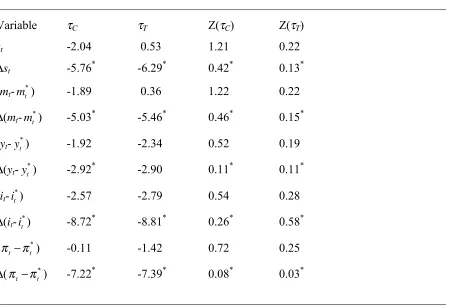
As a next step, we investigate the time series properties of the variables of interest. Spurious regression problem introduced by Yule (1926), and further analyzed by Granger and Newbold (1974), Phillips (1986) and Phillips and Durlauf (1986) indicate that using non-stationary time series steadily diverging from long-run mean causes to unreliable correlations within the regression analysis leading to unbounded variance process. However, for the mean, variance and covariance of a time series to be constant over time requires that conditional probability distributions of the series tend to be invariant with respect to the time, and if only so can the conventional procedures of OLS resgressions be applied using a stationary process for the variables. Therefore, at first by using the augmented Dickey-Fuller (ADF) unit root tests of Dickey and Fuller (1979, 1981) under the null hypothesis for the presence of a unit root against the stationary alternative hypothesis, we check for the stationarity condition of our variables and compare the estimated ADF statistics with the simulated MacKinnon (1991, 1996) critical values, which employ a set of simulations to derive asymptotic results and to simulate critical values for arbitrary sample sizes. For the case of stationarity, we expect that these statistics are larger than the MacKinnon critical values in absolute value and that they have a minus sign. The lags used for the ADF stationarity test are augmented up to a maximum of 10 lags and the choice of the optimum lag was decided on the basis of minimizing the Schwarz Information Criterion (SC). ‘*’ indicate the rejection of a unit root.
12
[image:13.595.75.524.157.464.2]null in the KPSS test. Yavuz (2004) highlights the properties of the ADF type and KPSS tests and tries to compare them by using Turkish stock exchange data:
Table 1: Unit Root Tests
___________________________________________________________________________ Variable τC τT Z(τC) Z(τT)
st -2.04 0.53 1.21 0.22 ∆st -5.76* -6.29* 0.42* 0.13*
(mt-mt*) -1.89 0.36 1.22 0.22
∆(mt-mt*) -5.03
*
-5.46* 0.46* 0.15*
(yt-y*t) -1.92 -2.34 0.52 0.19
∆(yt-y*t) -2.92
*
-2.90 0.11* 0.11*
(it-it*) -2.57 -2.79 0.54 0.28
∆(it-it*) -8.72
*
-8.81* 0.26* 0.58*
(π πt − t*) -0.11 -1.42 0.72 0.25
∆(π πt − t*) -7.22* -7.39* 0.08* 0.03*
___________________________________________________________________________
Above, τC and τT are the test statistics with allowance for only constant and constant&trend tems in the unit root tests, respectively, and Z(C) and Z(T) are the relevant KPSS statistics. ‘∆’ denotes the first difference operator. The results of ADF unit root tests reveal that the null hypothesis that there is a unit root cannot be rejected for all the variables in the level form, but inversely, for the first differences the stationary alternative hypothesis can be accepted. Likewise, the KPSS tests under the null hypothesis of stationarity indicate that all the variables are of difference-stationary form.
III. 2. Some Methodological Issues
13
(1981), the traditional large-scaled simultaneous equation macroeconometric models are not able to detect most econometric long-run relationships and lead to controversies as for the stability of structural relationships between macroeconomic aggregates. Also the classic paper by Nelson and Plosser (1982) reveal that many macroeconomic time series data have a stochastic trend plus a stationary component, that is, they are difference stationary processes, and following Enders (2004) we can state that numerious economic theories suggest the importance of distinguishing between temporary and permanent movements in a series. In this sense, economic theory assumes that at least some subsets of economic variables do not drift through time independently of each other and some combination of the variables in these subsets reverts to the mean of a stable stochastic process (Anderson et al., 1998).
Granger (1986) and Engle and Granger (1987) indicate that even though economic time series may be non-stationary in their level forms, there may exist some linear combination of these variables that converge to a long run relationship over time, which also requires that there must be Granger causality in at least one direction in an economic sense as one variable can help forecast the others. That is, if the series are individually stationary after differencing but a linear combination of their levels is stationary then the series are said to be co-integrated. In such a case, they cannot move too far away from each other in a theoretical sense (Dickey, Jansen and Thornton, 1991). Engle and Yoo (1987) using some Monte Carlo experiments estimate that forecasts taken from co-integrating relations will have a finite limiting forecast error variance leading to that they are tied together because the co-integrating relations must hold exactly in the long run (Hoffman and Rasche, 1996). However, as emphasized in Anderson et al. (1998), since the long-horizon forecast of the error correction term is always zero, incorporating co-integrating relationships for forecasting purposes may reduce mean square forecast error only at short horizons.
14
methodology, enabling also to testing that more than one stationary long-run equilibrium relation can be lying in the long-run variable space, take account of the non-stationarity characteristics of the most economic aggregate time series. Whereas, employing conventional estimation techniques based on an OLS estimation would not possibly lead to a constant mean and a finite variance and therefore diverge after a shock. In line with these developments in econometrics theory, contemporaneous economics theories make use of these estimation tools in constructing and testing the theories based on model specification issues conditioned upon econometrics.
III. 3. Johansen-Juselius Multivariate Co-integration Techniques
In order to test for a long-run stationary relationship derived from the variable space expressed above, we apply to the multivariate co-integration and vector error correction (VEC) techniques proposed by Johansen (1988) and Johansen and Juselius (1990). This methodology constructs an error correction mechanism among the same order integrated variables enabling that a stationary combination of the variables do not drift apart without bound even though all have been individually subject to a non-stationary I(d) process, therefore ruling out the possibility that estimated relationships tend to be spurious. Besides, this technique is superior to the regression-based techniques, e.g. Engle and Granger (1987) two-step methodology, for it enables researchers to capture all the possible stationary relationships lying within the long-run variable space. Following MacDonald and Taylor (1993), however, using ordinary least squares to estimate a co-integrating relationship for an
n-dimensioned vector does not clarify whether one is dealing with a unique co-integrating vector or a linear combination of the potential n-1 distinct co-integrating vectors that may be lying within the long-run variable space.
Let us assume a zt vector of non-stationary n endogenous variables and model this vector as
an unrestricted vector autoregression (VAR) involving up to k-lags of zt:
zt=Π1zt-1+Π2zt-2+ … + Πkzt-k+εt (9)
15
∆zt=Γ1∆zt-1+Γ2∆zt-2+ … +Γk-1∆zt-k+1+Πzt-k + εt (10)
where:
Γi = -I + Π1 + … + Πi (i = 1, 2, …, k-1) and Π = I - Π1 - Π2 - … - Πk (11)
Eq. 10 can be arrived at by subtracting zt-1 from both sides of Eq. 9 and collecting terms on zt-1
and then adding -(Π1 - 1)Xt-1 + (Π1 - 1)Xt-1. Repetition of this process and the collection of
terms would yield Eq. 10 (Hafer and Kutan, 1994). This specification of the system of variables carries on the knowledge of both the short- and the long-run adjustment to changes in zt, via the estimates of Γi and Π. Following Harris (1995), Π = αβ′ where α measures the
speed of adjustment coefficient of particular variables to a disturbance in the long-run equilibrium relationship and can be interpreted as a matrix of error correction terms, while β is a matrix of long-run coefficients such that β′zt embedded in Eq. 10 represents up to (n-1)
cointegrating relations in the multivariate model which ensure that zt converge to their
long-run steady-state solutions. Note that all terms in Eq. 10 which involve ∆zt-i are I(0) while Πzt-k
must also be stationary for εt ~ I(0) to be white noise of an N(0, σε2) process.
Dealing with the rank conditions, three alternative cases can be considered. If the rank of matrix equals zero, there would be no co-integrating relation between the endogenous variables, which means that there would be no linear combinations of the zt that are I(0)
leading to that Π would be an (nxn) matrix of zeros. In this case, a VAR model consisted of a set of variables in first differences thus carrying no long-run knowledge of any stationary relationship could be suggested to examine the variable system. If the Π matrix is of full rank when r = n, then all elements in zt would be stationary in their levels. Of special interest for us
here is the possibility that there exist r co-integrating vectors in zt-k~ I(0) and (n-r) common
stochastic trends when Π has reduced rank, i.e., 0 < r (n-1). That is, the first r columns of β are the linearly independent combinations of the endogenous variables settled in vector zt,
16
long-run stationary equilibrium process. Thus, this method is equivalent to testing which columns of α are zero (Harris, 1995). Gonzalo (1994) indicates that this method performs better than other estimation methods even when the errors are non-normal distributed or when the dynamics are unknown. Further, this method does not suffer from problems associated with normalisation (Johansen, 1995). We thus first determined the lag length of our unrestricted VAR model using sequential modified LR statistics employing small sample modification, which compare the modified LR statistics to the 5% critical values starting from the maximum lag and decreasing the lag one at a time until first getting a rejection. Considering the maximum lag of 8 for the unrestricted VAR model of quarterly frequency data, in our case reduction of system is first rejected when applying to 5 lag orders by the sequential modified LR statistics. Besides, the minimized Akaike information criterion suggests using the five lag orders. However, Schwarz (SC) and Hannan-Quinn (HQ) statistics suggest one lag order to be considered.
On this point, we should specify that for the appropriate lag length to ensure that the residuals are Gaussian, i.e.. they do not suffer from autocorrelation, non-normality, etc., considering the presence of co-integrating relationships used in the next sub-section, Cheung and Lai (1993) find that Monte Carlo experience carried out using data generating processes (DGPs) suggests that tests of co-integration rank are relatively robust to over-parametrizing, while setting too small a value of lag length such as lag length one or two generally suggested by SC statistics also producing serial correlation problem severely distorts the size of the maximum likelihood tests (Cheung and Lai, 1993; Harris, 1995). Gonzalo (1994) also reveals that the cost of over-parametrizing by including more lags in the maximum likelihood based error correction model (ECM) is small in terms of efficiency lost, but this is not the case if the ECM is underparametrized.
As a next step, we estimate the long run co-integrating relationships between the variables by using two likelihood test statistics known as maximum eigenvalue for the null hypothesis of r
versus the alternative of r+1 co-integrating relationships and trace for the null hypothesis of r
17
H0: λi = 0, i = r+1, …, n (12)
where only the first r eigenvalues are non-zero. This restriction can be imposed for different values of r and then the log of the maximised likelihood function for the restricted model is compared to the log of the maximised likelihood function of the unrestricted model and a standard LR test computed. Using the trace statistic we can test the null hypothesis:
1
2 log( ) log(1 )
n
trace i
i r
Q T
λ λ
= +
= − = −
∑
− and r = 0, 1, 2, …, n-2, n-1 (13)where Q = (restricted maximized likelihood / unrestricted maximised likelihood), T is the sample size. Another test of the significance of the largest λi is the maximal-eigenvalue statistic:
λmax = -T log (1-λr+1) and r = 0, 1 ,2, …, n-2, n-1 (14)
which tests that there are r co-integration vectors against the alternative that r+1 exist as expressed above.
18
that restricting the trend factor into the co-integration space is preferable. In line with these model specification issues, we assume that a long-run deterministic trend would be restricted in the co-integrating space, but no deterministic trend is allowed for the short-run dynamics.
In the next section we give the estimation results of the model including also a set of centered seasonal dummy variables included into the model, which sum to zero over a year as exogeneous variable. Johansen (1995) indicates that the linear term from the dummies in this way disappears and is taken over completely by the constant term, and only the seasonally varying means remain. For instance, the second quarter takes the value of 0.75 while the sum of the remaining three quarters’ dummies is -0.75.
III. 4. Estimation Results
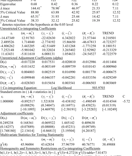
In line with data and econometric model specification issues highlighted so far, the TL/US$ exchange rate determination model is estimated using the multivariate co-integration methodology of the same order integrated variables. In Tab. 2 below which reports the results of Johansen co-integration test using max-eigen and trace tests based on critical values taken from Osterwald-Lenum (1992) are given the estimation results in which a constant and long-run deterministic trend are restricted but no deterministic trend is assumed for dynamic VEC model. So doing we leave the 2004Q1-2006Q4 period for out-of-sample forecasting purposes.
Rewriting the exchange rate equation under the assumption of r = 1:
st = 0.89(mt−mt*)- 1.52
*
(yt−yt) + 0.44
*
(it −it ) + 1.49
*
(π πt− t) + 0.01TREND + 5.72 (15)
19
Table 2: Co-integration Test
___________________________________________________________________________ Null hypothesis r=0 r≤1 r≤2 r≤3 r≤4
Eigenvalue 0.68 0.42 0.36 0.22 0.12
λtrace 144.41* 78.90* 46.97* 21.53 7.11 5% Critical Value 88.80 63.88 42.92 25.87 12.52
λmax 65.51* 31.93 25.44 14.42 7.11 5% Critical Value 38.33 32.12 25.82 19.39 12.52
*
denotes rejection of the hypothesis at the 0.05 level Unrestricted Co-integrating Coefficients
st (mt−mt*)
*
(yt−yt)
*
(it −it )
*
(π πt − t) TREND -14.47349 12.91783 -22.02630 6.342022 21.57344 0.210501 2.489526 1.714840 -2.774192 15.86650 -46.67813 -0.723257 -4.806262 3.443205 -42.51449 3.431268 -1.771258 0.180151 7.252148 -5.901042 10.32024 3.265402 12.92902 -0.213329 11.63431 -5.811610 6.008131 1.054633 -24.54527 -0.722579 Unrestricted Adjustment Coefficients (alpha)
D(s) -0.017220 0.017531 -0.020810 -0.012986 -0.011404 D(mt −mt*) -0.011632 -0.003169 -0.009759 0.010143 -0.000960 D(yt−yt*) 0.004803 0.002519 0.016990 0.001770 -0.000675 D(it−it*) -0.099848 -0.046357 -0.042281 -0.033356 -0.029249 D(π πt − t*) -0.028303 0.015654 0.003541 -0.006503 0.003069 1 Co-integrating Equation: Log likelihood 503.9703
Standard errors in ( ) & t-statistics in [ ]
st (mt−mt*)
*
(yt−yt) (it −it*) (π πt − t*) TREND C 1.000000 -0.892517 1.521838 -0.438182 -1.490549 -0.014544 -5.72
(0.08829) (0.34047) (0.16971) (0.45823) (0.01319) [-10.1095] [4.46979] [-2.58191] [-3.25283] [-1.10249] Adjustment coefficients
D(st) D(mt−mt*) D
*
(yt−yt) D
*
(it −it ) D
*
(π πt − t) 0.249238 0.168361 -0.069522 1.445142 0.409638 (0.14257) (0.07889) (0.08008) (0.45231) (0.09749) [1.748180] [2.13414] [-0.86813] [3.19504] [4.20187] Multivariate Statistics for Testing Stationarity
st (mt−m*t)
*
(yt −yt) (it−it*) (π πt− t*)
χ2
(4) 45.96004 43.62834 37.96759 40.76771 38.49888 Homogeneity and Symmetry Restrictions on Co-integrating Coefficients
b(1,1)=1, b(1,2)=-1, b(1,3)=1, b(1,5)=-1, χ2(3)=4.27216 χ2(3)-table=7.81473
b(1,1)=1, b(1,2)=-1, b(1,3)=1, b(1,4)=-1, b(1,5)=-1, χ2(4)=9.41221 χ2(4)-table=9.48773 ___________________________________________________________________________
20
When we normalize the first vector on the nominal exchange rate in Eq. 15 we find a theoretically plausible co-integrating equation. The relative money supply has a positive and relative real income has a negative significant long-run relationship with nominal exchange rate. These findings are common for all the models explaining monetary exchange rate determination. Besides, inflation differentials lead to a depreciation of the domestic currency as expected. The interest differential variable has a positive and significant sign recalling the FPMM of exchange rate determination. Thus, no support is given to the assumption that relative interest differential in favor of domestic interest rates leads to an appreciation of the domestic currency. These results are in line with the findings of Bahmani-Oskooee and Kara (2000) but contradict Dulger and Cin (2002). Goldberg (2000) relates the positive sign of interest rate in the monetary model also to the under-or-overshooting of the exchange rate under perfect or imperfect capital mobility.
21
The hypothesis sp(H5) ⊂ sp(β) presented by Johansen and Juselius (1992) assumes r1 of the r
co-integrating relations known as specified by the matrix H5. The remaining r2 relations are
choosen without restrictions. This type of hypothesis for r = 1 differs from widely used testing procedure of the Dickey-Fuller type of univariate testing in the sense that the former as a χ2 test hypothesizes stationarity as the null hypothesis, whereas the usual latter univariate tests formulate the null of nonstationarity. Our former estimation results from the ADF and KPSS unit root testing procedures above, which may yield incorrect inferences when the data generating process has shifted by the time, are verified by the Johansen-Juselius type of testing stationarity in the sense that no variable alone can represent a stationary relationship in the co-integrating vector.
Finally, we accept the null hypothesis of homogeneity and symmetry restrictions applied in Tab. 2. If we explicitly write down these equations:
st = (mt−m*t)-
*
(yt−yt) + 0.68( *)
t t
i −i + ( *)
t t
π π− - 0.00223TREND + 5.16 (16)
producing χ2(3) = 4.27216 against χ2(3)-table = 7.81473, and:
st = (mt−m*t)-
*
(yt−yt) + ( *)
t t
i −i + ( *)
t t
π π− - 0.00416TREND + 4.97 (17)
producing χ2(4) = 9.41221 against χ2(4)-table = 9.48773. We must note that no VEC residual serial correlation problem occurs using LM-statistics LM(1)=20.56682 (0.7165) and LM(4)=25.66830 (0.4255) under the null of no serial correlation of the 1st or 4th order using prob. values in parenthesies from χ2 with 25 d.o.f. Under the null of no heteroskedasticity or no misspecification VEC residual heteroskedasticity test gives that χ2(825)=833.1149 using the prob value of 0.4147. However, under the null hypothesis of multivariate normal residuals VEC residual normality test produces excess kurtosis and non-normality using skewness
χ2
22
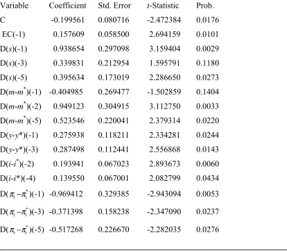
[image:23.595.71.485.208.569.2]Having established the long run co-integrating equilibrium model, we now estimate the parsimonious VEC model whitening the error structure. We include two variables which have probs. above 5% due to multicollinearity problems:
Table 3: Parsimonious VEC Model
___________________________________________________________________________ White Heteroskedasticity-Consistent Standard Errors &Covariance
Variable Coefficient Std. Error t-Statistic Prob. C -0.199561 0.080716 -2.472384 0.0176 EC(-1) 0.157609 0.058500 2.694159 0.0101 D(s)(-1) 0.938654 0.297098 3.159404 0.0029 D(s)(-3) 0.339831 0.212954 1.595791 0.1180 D(s)(-5) 0.395634 0.173019 2.286650 0.0273 D(m-m*)(-1) -0.404985 0.269477 -1.502859 0.1404 D(m-m*)(-2) 0.949123 0.304915 3.112750 0.0033 D(m-m*)(-5) 0.523546 0.220041 2.379314 0.0220 D(y-y*)(-1) 0.275938 0.118211 2.334281 0.0244 D(y-y*)(-3) 0.287498 0.112441 2.556868 0.0143 D(i-i*)(-2) 0.193941 0.067023 2.893673 0.0060 D(i-i*)(-4) 0.139550 0.067001 2.082799 0.0434 D( *
t t
π π− )(-1) -0.969412 0.329385 -2.943094 0.0053
D( *
t t
π π− )(-3) -0.371398 0.158238 -2.347090 0.0237
D( *
t t
π π− )(-5) -0.517268 0.226670 -2.282035 0.0276
___________________________________________________________________________
23
III. 5. Out-of-Sample Predictability
We now try to compare the out-of-sample forecasting performances from the benchmark random walk (RW) and random walk with drift (RWt) models, for which following Enders (2004) the latter is governed by two nonstationary process, i.e. a linear deterministic trend and a stochastic trend, against our fundamental based monetary exchange rate error correction model (FBMM). The out-of sample forecasts are evaluated for the 2004Q1-2006Q4 period. We compute fully dynamic predictions in this period from one to eleven forecast periods of the quarterly observations so that previously forecasted values are used in forming the forecasts of the current period. Thus, such a forecasting methodology will differ from static forecasts which calculate a sequence of one-step forecasts using the actual rather than forecasted values in estimation process. Following Mark(1995) and Neely and Sarno (2002), we will use the Theil’s U statistics, that is, the ratio of root mean squared errors (RMSEs) from two competing models considering monetary versus random walk with/without drift models. A ratio less than one would give support to the superior forecasting performance of the fundamental based model, while a ratio greater than one would support the forecasting ability of RW model when compared with the fundamental based monetary model. The results can be seen in Tab. 4 and Tab. 5 below.
Tab. 4 and Tab. 5 reveal that fundamental based monetary model out-performs the benchmark random walk models for the forecast horizons of one to nine or one-to ten quarters and then random walk model has superiority in forecasting against the fundamental based model. These results indicate that assuming the knowledge from co-integrating relationship tends to improve the success of forecasting inside a 2.5 years forecasting horizon.
IV. CONCLUDING REMARKS
24
TABLE 4: FBMM / RW OUT-OF-SAMPLE FORECASTING COMPARISONS
___________________________________________________________________________ Forecast
horizon 1 2 3 4 5 6 7 8 9 10 11 FBMM / RW 0.77 0.63 0.57 0.65 0.68 0.67 0.72 0.82 0.91 1.04 1.22 ___________________________________________________________________________
TABLE 5: FBMM / RWt OUT-OF-SAMPLE FORECASTING COMPARISONS
___________________________________________________________________________ Forecast
horizon 1 2 3 4 5 6 7 8 9 10 11 FBMM / RW 0.69 0.55 0.50 0.56 0.59 0.58 0.62 0.70 0.78 0.87 1.02 ___________________________________________________________________________
stylized facts based on such researches, and policies should be constructed in line with the requirements extracted through testing the economics theory.
In our paper, we try to investigate the exchange rate determination mechanism for the Turkish economy. Our empirical findings following a large literature review explaining monetary model exchange rate determination and employing multivariate Johansen-Juselius type co-integrating approach indicate that TL/US$ nominal exchange rate is co-integrated with the fundamentals suggested by economics theory. We find that short-run deviations from the fundamental-based equilibrium course of the nominal exchange rate have permanent effects on the long-run equilibrium exchange rate and so have been stemmed from the existence of some form of hysteresis effects dominated in the nominal exchange rate. Results obtained also indicate that fundamental based monetary model out-performs the benchmark random walk with/without drift models for the forecast horizons between one to nine and one to ten quarters thus leading us to the conclusion that knowledge from co-integrating relationship tends to improve the success of forecasting performance for the exchange rate determination model.
25
researchers confirm whether estimation results in this paper are in fact of the stylized facts for the Turkish economy.
REFERENCES
Abhyankar, A., Sarno, L. and Valente, G. (2005). Exchange rates and fundamentals: evidence on the economic value of predictability, Journal of International Economics, 66, 325-348.
Anderson, R. G., Hoffman, D. and Rasche, R. H. (1998). A vector error correction forecasting model of the U.S. economy, The Federal Reserve Bank of St Louis Working Paper, 98-008A, May.
Bahmani-Oskooee, M. and Kara, O. (2000). Exchange rate overshooting in Turkey,
Economics Letters, 68, 89- 93.
Berkowitz, J. and Giorgianni, L. (2001). Long-horizon exchange rate predictability?, Review of Economics and Statistics, 83/1, 81-91.
Bilson, J.F.O. (1978a). Rational expectations and the exchange rate, In: Frenkel, J.A. and Johnson, H.G. (eds.), The Economics of Exchange Rates: Selected Studies, New York: Addison-Wesley, 201-223.
Bilson, J.F.O. (1978b). The monetary approach to the exchange rate: some empirical evidence, IMF Staff Papers, 25, 48-75.
Cheung, Y.-W. and Chinn, M. D. (1998). Integration, cointegration and the forecast consistency of structural exchange rate models, Journal of International Money and Finance, 17, 813-830.
26
Chinn, M.D. and Meese, R.A. (1995). Banking on currency forecasts: is change in money predictable?, Journal of International Economics, 38, 161-178.
Civcir, I. (2003a). Before the fall was the Turkish lira overvalued, Eastern European Economics, 41/2, 69-90.
Civcir, I. (2003b). The monetary model of the exchange rate under high inflation: the case of Turkish Lira-US Dollar, Finance A Uver, 53/3-4, 113-129.
Civcir, I. (2003c). The monetary models of the exchange rate: long-run relationships, short-run dynamics and forecasting, Eastern European Economics, 41/6 43-69.
DeJong, D. N., Nankervis, J. C., Savin, N. E. and Whiteman, C. H. (1989). Integration versus trend-stationarity in macroeconomic time-series, University of Iowa Working Paper Series, No. 89/31, December.
Dickey, D.A. and Fuller, W.A. (1979). Distribution of the estimators for autoregressive time series with a unit root, Journal of the American Statistical Association, 74, 427-431.
Dickey, D.A. and Fuller, W.A. (1981). Likelihood ratio statistics for autoregressive time series with unit roots, Econometrica, 49, July, 1057-1072.
Dickey, D. A., Jansen, D. W. and Thornton, D. L. (1991). A primer on cointegration with an application to money and income, The Federal Reserve Bank of St. Louis Review, March/April, 58-78.
Doornik, J.A., Hendry, D.F. and Nielsen, B. (1998). Inference in cointegrating models: UK M1 revisited, Journal of Economic Surveys, 12/5, 533-572.
27
Dulger, F. and Cin, M.F. (2002). Monetary approach to determining exchange rate dynamics in Turkey and a test for cointegration (in Turkish), METU Studies in Development, 29/1-2, 47-68.
Enders, W. (2004). Applied Econometric Time Series, Second Ed., John Wiley & Sons, Inc.
Engle, R. F. and Granger, C. W. J. (1987). Co-integration and error correction: representation, estimation, and testing, Econometrica, 55, 251-276.
Engle, R. F. and Yoo, B. S. (1987). Forecasting and testing in cointegrated systems, Journal of Econometrics, 35, 143-159.
Erlat, H. (2003). The nature of persistence in Turkish real exchange rates, Emerging Markets Finance and Trade, 39/2, 70-97.
Frankel, J.A. (1979). On the mark: a theory of floating exchange rates based on real interest differentials, American Economic Review, 69/4, 610-622.
Frenkel, J.A. (1976). A monetary approach to the exchange rate: doctrinal aspects and empirical evidence, Scandinavian Journal of Economics, 78/2, 200-224.
Gokcan, A. and Ozmen, E. (2002). Do PPP and UIP need each other in a financially open economy? the Turkish evidence, ERC Working Papers in Economics, 01/01, May.
Goldberg, M. D. (2000). On empirical exchange rate models: what does a rejection of the symmetry restriction on short-run interest rates mean?, Journal of International Money and Finance,19, 673-688.
Gonzalo, J. (1994). Five alternative methods of estimating long-run equilibrium relationships,
Journal of Econometrics, 60, 203-233.
Granger, C. W. J. (1986). Developments in the study of cointegrated economic variables,
28
Granger, C.W.J. and Newbold, P. (1974). Spurious regressions in economics, Journal of Econometrics, 2/2, 111-120.
Groen, J.J.J. (2000). The monetary exchange rate model as a long-run phenomenon, Journal of International Economics, 52, 299-319.
Harris, R.I.D. (1995). Using Cointegration Analysis in Econometric Modelling, Prentice Hall.
Hendry, D. F. (1986). Econometric modelling with cointegrated variables: an overview,
Oxford Bulletin of Economics and Statistics, 48/3, 201-212.
Hoffman, D. L. and Rasche, R. H. (1996). Assessing forecast perfomance in a cointegrated system, Journal of Applied Econometrics, 11/5, 495-517.
Hooper, P. and Morton, J.E. (1982). Fluctuations in the dollar: a model of nominal and real exchange rate determination, Journal of International Money and Finance, 1, 39-56.
Johansen, S. (1988). Statistical analysis of cointegration vectors, Journal of Economic Dynamics and Control, 12, 231-254.
Johansen, S. (1992). Determination of cointegration rank in the presence of a linear trend,
Oxford Bulletin of Economics and Statistics, 54/3, 383-397.
Johansen, S. (1995), Likelihood-based Inference in Cointegrated Vector Autoregressive Models, Oxford University Press.
Johansen, S. and Juselius, K. (1990). Maximum likelihood estimation and inference on cointegration-with applications to the demand for money, Oxford Bulletin of Economics and Statistics, 52, pp.169-210.
29
Karfakis, C. (2006). Is there an empirical link between the dollar price of the euro and the monetary fundamentals?, Applied Financial Economics, 16, 973-980.
Kesriyeli, M. (1994). Policy regime changes and testing for the Fisher and UIP hypothesis: the Turkish experience, CBRT Research Department Discussion Paper, No. 9411, December.
Kilian, L. (1999). Exchange rates and monetary fundamentals: what do we learn from long-horizon regressions?, Journal of Applied Econometrics, 14/5, 491-510.
Kwiatkowski, D., Phillips, P.C.B., Schmidt, P. and Shin, Y. (1992). Testing the null hypothesis of stationary against the alternative of a unit root, Journal of Econometrics, 54, 159-178.
Lucas, R.E. (1981). Econometric policy evaluation: a critique, In: Lucas, R.E. (ed.), Studies in Business-Cycle Theory, MIT Press, 104-130.
Lütkepohl, H. (1991). Introduction to Multiple Time Series Analysis, New York: Springer-Verlag.
MacDonald, R. and Marsh, I.W. (1997). On fundamentals and exchange rates: a Casselian perspective, Review of Economics and Statistics, 79/4, 655-664.
MacDonald, R. and Taylor, M.P. (1993). The monetary approach to the exchange rate rational expectations, long-run equilibrium, and forecasting, IMF Staff Papers, 40/1, 89-107.
MacKinnon, J.G. (1991). Critical values for cointegration tests, In: R. F. Engle and C. W. J. Granger (eds.), Long-run Economic Relationships: Readings in Cointegration, Ch. 13, Oxford: Oxford University Press.
30
Mark, N. C. (1995). Exchange rates and fundamentals: evidence on long-horizon predictability, American Economic Review, 85/1, 201-218.
Mark, N.C. and Sul, D. (2001). Nominal exchange rates and monetary fundamentals evidence from a small post- Bretton woods panel, Journal of International Economics, 53, 29-52.
McNown, R. and Wallace, M.S. (1994). Cointegration tests of the monetary exchange rate model for three high- inflation economies, Journal of Money, Credit and Banking, 26/3, 396-411.
Meese, R. A. and Rogoff, K. (1983). Empirical exchange rate models of the seventies: do they fit out of sample?, Journal of International Economics, 14/1-2, 3-24.
Metin, K. (1994). A test of long-run purchasing power parity and uncovered interest parity: Turkish case, Bilkent University Discussion Papers, No. 94/2.
Moosa, I. A. (2000). A structural time series test of the monetary model of exchange rates under the German hyperinflation, Journal of International Financial Markets, Institutions and Money, 10, 213-223.
Mussa, M. (1976). The exchange rate, the balance of payments and monetary and fiscal policy under a regime of controlled floating, Scandinavian Journal of Economics, 78/2, 229-248.
Neely, C.J. and Sarno, L. (2002). How well do monetary fundamentals forecast exchange rates?, FRB of St. Louis Review, September/October, 51-74.
Nelson, C. and Plosser, C. (1982). Trend and random walks in macroeconomic time series: some evidence and implications, Journal of Monetary Economics, 10, 130-162.
Nwafor, F.C. (2006). The naira-dollar exchange rate determination: a monetary perspective,
31
Osterwald-Lenum, M. (1992). A note with quantiles of the asymptotic distribution of the maximum likelihood cointegration rank test statistics, Oxford Bulletin of Economics and Statistics, 54, 461-472.
Ozdemir, Z.A. (2004). Mean reversion in real exchange rate: empirical evidence from Turkey, 1980-1999, METU Studies in Development, 31, 243-265.
Pesaran, H. M. and Shin, Y. (1999). An autoregressive distributed lag modelling approach to co-integration analysis, In: Strom, S. (ed.), Econometrics and Economic Theory in the 20th Century: The Ragnar Frish Centennial Symposium, Cambridge University Press, Cambridge.
Pesaran, H. M., Shin, Y. and Smith, R. J. (2001). Bound testing approaches to the analysis of level relationships, Journal of Applied Econometrics, 16, 289-326.
Phillips, P. (1986). Understanding spurious regressions in econometrics, Journal of Econometrics, 33, 311-40.
Phillips, P. and Durlauf, S. (1986). Multiple time series regression with integrated process,
Review of Economic Studies, 53, 473-495.
Rapach, D.E. and Wohar, M.E. (2002). Testing the monetary model of exchange rate determination: new evidence from a century of data, Journal of International Economics, 58, 359-385.
Rapach, D.E. and Wohar, M.E. (2004). Testing the monetary model of exchange rate determination: a closer look at panels, Journal of International Money and Finance, 23, 867-895.
32
Straus-Kahn, M. O. (1991). Error correction models and cointegration in the Bank of France’s econometric works, In: Central Bank of the Republic of Turkey (ed.), The Use of Econometric
Models in Central Banks’ Decision Making Problems, Papers Presented at a Workshop held
in Ankara, Turkey on 11-14 September 1989, Ankara, August, 15-88.
Telatar, E. and Kazdagli, H. (1998). Re-examine the long-run purchasing power parity hypothesis for a high inflation country: the case of Turkey, Applied Economics Letters, 5, 51-53.
Yavuz, N.C. (2004). KPSS and ADF tests in determining stationarity: an application to ISE National-100 index (in Turkish), Journal of Istanbul University Faculty of Economics, 54/1, 239-247.
Yazgan, M.E. (2003). The purchasing power parity hypothesis for a high inflation country: a re-examination of the case of Turkey, Applied Economics Letters, 10/3, 143-147.