Calculation of the Properties of Reentrant
Cylindrical Cavity Resonators
Richard G. Carter
, Senior Member, IEEE
, Jinjun Feng
, Member, IEEE
, and Ulrich Becker
Abstract—The lowest resonant frequencies of reentrant cylin-drical cavity resonators are calculated using the method of mo-ments to obtain upper and lower bounds. The accuracy and conver-gence of the results are investigated and the factors and shunt impedances calculated. A simple empirical assumption about the choice of basis functions leads to results that are of good accuracy and readily computed. The results obtained are compared with those of experiment and from calculations using MAFIA and Mi-crowave Studio.
Index Terms—Cavity resonators, frequency, method of mo-ments, shunt impedance, factor, upper and lower bounds.
I. INTRODUCTION
T
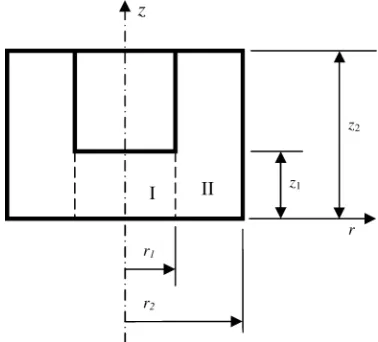
HE PROPERTIES of cavity resonators (resonant fre-quency, factor, and shunt impedance) are commonly calculated using finite-difference time-domain, finite-element, and other similar methods [1]. A variety of computer codes are available for this purpose and the power of modern computers means that the properties of many cavities can be calculated quickly and with good accuracy. However, some commonly encountered geometries, such as the cylindrical reentrant cavity shown in Fig. 1, include sharp edges, which are difficult to model accurately using these methods. It is usually necessary to use very large numbers of mesh cells to obtain good accuracy and the computational time becomes much longer.In an alternative approach, the electric and magnetic fields in each region of the cavity are represented by infinite series of basis functions, which are then matched by the imposition of a continuity condition at . This method was proposed for the reentrant cavity by Hansen [2] who assumed an approx-imate variation of the electric field on the boundary between them. The resonant frequency of the lowest TM mode was de-termined by matching the magnetic fields at the point . In a further development of this method, Chu and Hansen [3] showed that upper and lower bounds to the resonant frequency could be obtained from assumed variations of the electric and magnetic fields on the boundary by requiring that the flux of the reactive Poynting vector should be continuous at . This
Manuscript received May 31, 2007; revised September 3, 2007. This work was supported in part by the Particle Physics and Astronomy Research Council, U.K., under Grant PPA/G/S/2000/00055.
R. G. Carter is with the Engineering Department, Lancaster University, Lan-caster LA1 4YR, U.K. (e-mail: [email protected]).
J. Feng is with the Vacuum Electronics National Laboratory, Beijing Vacuum Electronics Research Institute, Beijing 100016, China (e-mail: [email protected]).
U. Becker is with the Technical Support Group, CST GmbH, D-64289 Darm-stadt, Germany (e-mail: [email protected]).
[image:1.594.331.520.164.335.2]Digital Object Identifier 10.1109/TMTT.2007.909750
Fig. 1. Cross section of a reentrant cylindrical cavity.
method is closely related to that used by Schwinger to determine upper and lower bounds for the admittances of discontinuities in waveguides [4], [5]. A further important step was taken by Taylor [6] who showed that it is not necessary to assume the forms of the electric and magnetic fields. Instead, the field ex-pansions in the two regions can be linked by the continuity equa-tions to give a determinant whose value is zero at the resonant frequency. It has been shown [7], [8] that this process can lead to upper and lower bounds to the frequency and is effectively a variational method. Since the method reduces the problem to a matrix equation, it falls within the general class of moment methods [9].
The problem of computing the resonant frequency of the cavity shown in Fig. 1 has been addressed by many other au-thors, see, e.g., [10]–[14] and the references therein. However, Taylor’s method is the best one available for this problem because the computation of upper and lower bounds to the resonant frequency means that the accuracy of the solution is always known. This method is, therefore, valuable for the rapid and accurate computation of the properties of reentrant cavities and for providing a method by which the accuracy of results obtained by other methods can be checked. It can also be used to compute the properties of any resonant structure, which can be divided into two or more simple regions in which the fields can be expressed in terms of basis functions, which satisfy Maxwell’s equations and the external boundary conditions [7], [8]. The purpose of this paper is to examine the convergence of Taylor’s method and to show how it can be used to obtain accurate values for the resonant frequencies, factors, and shunt impedances of a wide range of cavities. We shall see that good results can be obtained by retaining only a few terms in
the series expansions of the fields when an empirical rule is applied.
II. THEORY
The theory of the method presented here is based on that de-scribed by Taylor, but uses matrix algebra. This makes it easier to understand and apply. In region I, the axial component of and the azimuthal component of , which satisfy the boundary conditions on the axis, may be written as [6]
(1) and
(2)
where the functions are defined in the Appendix, the prime denotes differentiation with respect to the argument
(3) and
(4) where . Now, when , let
(5)
(6)
where and are constant coefficients. Eliminating the co-efficients between (1), (2), (5), and (6), we obtain
(7) where and are column vectors of the coefficients in (5) and (6) and is a diagonal matrix whose elements are defined in the Appendix.
A similar equation can be derived for region II as
(8) where the elements of are defined in the Appendix and and are column vectors of the coefficients of the Fourier expansions of and in region II at analo-gous to those in (5) and (6).
The condition that is continuous at for and if is
if if
(9) where . When both sides of (9) are multiplied by and integrated from to , we obtain the matrix equation
(10)
where the matrix is defined in the Appendix. Similarly the continuity condition for at is
when
(11) When both sides of (11) are multiplied by and inte-grated from to , we obtain the matrix equation
(12) where the matrix is defined in the Appendix. It should be noted that the boundary condition for when is auto-matically satisfied by the distribution of the surface current.
It is now a simple matter to eliminate all the column vectors of the coefficients, except from (7), (8), (10), and (12) to obtain
(13) so that the eigenvalue is the solution of
(14) where is the unit matrix. This is equivalent to the solution obtained by Taylor [6] and Jaworski [14] (but note that the factor of 2 in [14, eq. (17)] is incorrect and should be replaced by 2). If, alternatively, the column vector is retained, we find that
(15) The derivations of (13)–(15) assume that both series of basis functions contain an infinite number of terms. In practice, the series must be terminated at and in regions I and II, respectively. Taylor [6] states that when the inner coefficients are eliminated, there is a discontinuity in at , leading to an upper bound for , and that the elimination of the outer coefficients leads to a discontinuity in and to a lower bound for . The existence of upper and lower bounds is said to be a consequence of regarding the truncated series of basis functions as a trial function in the variational sense. However, this explanation cannot be correct because when the same choice of and is used in both (13) and (15), the same value of is computed in each case. It is, therefore, necessary to examine more closely the relationship between the method of moments and the variational method implied by the truncation of the series.
III. VARIATIONALMETHOD
The variational method for this problem can be established in a simpler manner than in [7] and [8] by applying Poynting’s theorem [15] separately to the two regions. If the electric field is taken to vary with time as , then in region I,
(16)
defined and in terms of basis functions, which satisfy the external boundary conditions, the integral must be 0, except on . A similar equation can be written for region II. These equations may be added together to give the rate of change with time of the total stored energy in the cavity as
(17) where the integration is taken over the surface at . The negative sign in the integrand is necessary because the flux of the Poynting vector in (16) is defined in terms of the outward normal for the region. Now the left-hand side of (17) must be 0 at all times for the oscillations in a lossless cavity. When and are exact solutions to the problem, their tangential components are continuous when and the integral in (17) is identically 0. Let us now assume that the fields in the two regions are de-fined by two series of basis functions as above and choose to truncate the series in the inner region when . If we re-quire that the continuity condition (9) is satisfied, then an infinite number of terms is required in the outer region. The coefficients of the magnetic fields in the two regions are given by (7) and (8), and we note that these depend upon . There is now a dis-continuity in when and the continuity condition (11) cannot be satisfied. We may, however, impose some other, ap-proximate, continuity condition and an approximate value of is then determined. Following Schwinger and Saxon [4], let us choose that the flux of the reactive Poynting vector is continuous at . Equation (17) then shows that the total stored energy in the cavity is constant as, physically, it must be. Other possible choices of approximate continuity condition do not guarantee this. The flux of the reactive Poynting vector out of region I is given by
(18)
We now make use of (5) and (6) and note that the basis functions are mutually orthogonal so that
(19) where the expansion has been terminated at . In region II, the series is infinite and we have
(20)
We use (10) to express (20) in terms of as
(21)
so that the approximate continuity condition is
(22) Note that this expression is quadratic in the coefficients , which are, as yet, undetermined. Their values can be found by treating them as variational parameters and requiring that the value of should be stationary for small variations of them. Thus,
(23)
The first term is 0 when is stationary and the values of and are then the solution of the set of equations obtained by equating the second term in (23) to 0. It can be shown, after some manipulation, that this condition, which is a linear function of the coefficients, is identical to (13). Thus, the truncation of the series in , while retaining an infinite number of terms in the series in , leads to a stationary value of .
The same procedure may be carried out when the series for in the outer region is truncated at , while retaining an infinite number of terms in the inner region. The condition that should be stationary is then (15). Chu [8] has shown that the two values of determined in this way must be different and are upper and lower bounds to the exact solution. Thus, the method of moments naturally leads to upper and lower bounds for through the truncation of the series of basis functions in either region. We see that the explanation offered by Taylor [6] is misleading and that it is the method of truncation, and not the choice of coefficients to be retained, which leads to upper and lower bounds. These bounds are absolute limits and make it possible to determine the resonant frequency of the cavity with known accuracy.
IV. IMPLEMENTATION
The method described in Section III was implemented using Mathcad 13.1The solutions to (14) were found using the secant
method, which was terminated when the fractional error in was less than 10 . Once had been determined, the eigen-vector was obtained from (13) using the Mathcad function
eigenvecwith an eigenvalue of unity. The eigenvector was nor-malized to a gap voltage at . The other column vectors of coefficients for the electric and magnetic fields were obtained from (7), (8), and (10) so that the electric and magnetic fields
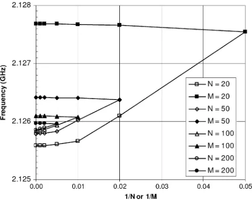
Fig. 2. Convergence of frequencies computed for a cavity for whichr =
6:004mm,r = 42:29mm,z = 7:958mm, andz = 22:792mm.
throughout the cavity could be computed to the level of approx-imation determined by the choices of and . The stored en-ergy and the energy loss per cycle were obtained by inte-grations over the volume of the cavity and over its surface so that the factor could be calculated. The results presented below as-sumed that the cavities were made of copper with conductivity 5.7 10 S m . Finally, the ratio of the shunt impedance to
was calculated using [16]
(24) where is the resonant frequency. The calculations usually take a few seconds on a PC with a 3-GHz Pentium 4 processor and 1 Gb of RAM.
V. CONVERGENCE OF THEMETHOD
The convergence of the method outlined above was studied using a cavity for which the frequency had been computed by Jaworski [14]. Fig. 2 shows that the resonant frequencies com-puted for constant decreased smoothly to a lower bound as was increased. Similarly, the resonant frequencies computed for constant increased smoothly to an upper bound as was increased. It can also be seen that the bounds obtained are nested within one another so that they are truly upper and lower bounds, as expected. In each case, the calculations were taken to (or ) and the infinite limits found by linear extrapola-tion. It may be noted that when , the frequency is always close to the upper bound. Fig. 3 shows the convergence of the infinite limits to the upper and lower bounds as the number of terms in the truncated series was progressively increased. When (or ) the bounds were 2.12588 and 2.12591 GHz giving a frequency of 2.1259 GHz to an accuracy of four dec-imal places. Fig. 3 also shows the lower bound results obtained by Jaworski [14] who was apparently unaware of the possibility of obtaining an upper bound. In his results, the maximum value of was 10 and linear extrapolation was used to obtain a res-onant frequency of 2.1276 GHz, which is in error by approxi-mately 0.08%. The difference between this result and those
[image:4.594.306.552.65.232.2]ob-Fig. 3. Convergence of the upper and lower bound frequencies for the same cavity as Fig. 2 with results from Jaworski [14].
Fig. 4. Convergence of the upper and lower bounds forN = 8andM = 24.
tained here was probably caused by not using a large enough value of (the value used was not stated). Fig. 2 shows that this would lead to an overestimate of the frequency, as observed. The method described here can give as high an accuracy as may be desired by suitable choices of and , but care is needed to ensure that proper convergence has been obtained.
VI. APPROXIMATEMETHOD
[image:4.594.305.553.271.451.2]Fig. 5. Convergence of the approximate frequency.
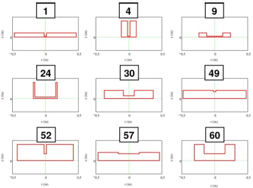
Fig. 6. Shapes of the test cavities.
fixing and increasing , as shown in Fig. 4. When and , the frequency is 2.1258 GHz to an ac-curacy of 1.4 MHz and 0.9 MHz. In practice, the accuracy of the result is greater than this because it lies almost midway between the bounds. Fig. 5 shows the results obtained using the approximate method for values of . The frequency was computed using in this way up to and it was found that, for , the result is 2.1259 GHz to an accuracy of four decimal places. Thus, the frequency computed when is actually accurate to 0.004%.
To evaluate the usefulness of the approximate method, nine very different cavities were selected from the set described by Hamilton et al.[17], which were also used by Fujisawa [18]. Since the shape of a cavity can be described by three normal-ized dimensions, the objective was to investigate all combina-tions of the extreme values of these together with one case in the center of the range. The shapes of the cavities are shown in Fig. 6 where the numbering corresponds to that used by Fuji-sawa. The resonant frequency and of each cavity were computed to eight significant figures with . In every case, the results were found to have converged to at least five significant figures when . A study of the dif-ferences between the results for and those for
showed that, in almost every case, the difference was less than 0.005%. The exceptions were cavities 4 and 52 in which is
[image:5.594.301.552.230.313.2]Fig. 7. Difference between the resonant frequencies of the test cavities com-puted with Microwave Studio and those obtained whenN = 8.
Fig. 8. Difference between theQfactors of the test cavities computed with Microwave Studio and those obtained whenN = 8.
Fig. 9. Difference between theR=Qof the test cavities computed with Mi-crowave Studio and those obtained whenN = 8.
small compared with and is appreciably less than . For those cavities, the differences were less than 0.01%, except for cavity 52 ( : 0.016%, : 0.011%). Thus, the properties of any cavity whose shape lies within the range of those computed can be calculated with an error of less than 0.01% using the ap-proximate method and .
VII. COMPARISONWITHOTHERMETHODS
The properties of the cavities in Fig. 6 were computed using Microwave Studio (MWS)2with the default setting of automatic
mesh refinement, which seeks the frequency to an accuracy of better than 1%. The differences between these results and those obtained with the approximate method are shown in Figs. 7–9. The differences are less than 1.0% for the fre-quency, 2.2% for the factor, and 5.7% for . The frequen-cies and factors show signs of systematic errors of around 0.5% and 1.4%, respectively. To investigate the comparison between the methods in more detail, results were computed for
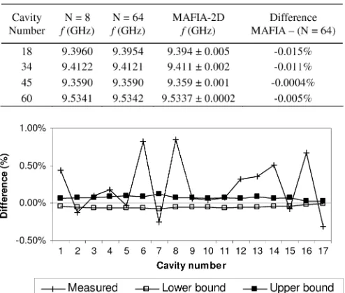
[image:5.594.39.289.234.420.2] [image:5.594.307.550.359.458.2]TABLE I
COMPARISONBETWEENRESULTSFROMMAFIA-2DAND
[image:6.594.42.289.102.312.2]FROM THEAPPROXIMATEMETHOD
Fig. 10. Difference between measured and calculated frequencies.
four cavities using MAFIA-2D, which employs the same algo-rithm as Microwave Studio, but which assumes cylindrical sym-metry. The first three of these were selected because the dif-ferences between the results obtained by the two methods had been particularly large in previous tests. The results in Table I show excellent agreement. The resonant frequency of cavity 60 calculated using MAFIA-2D and extrapolated to an infinite number of mesh nodes was 9.5339 GHz. Calculations using MWS and more than 2 million mesh points gave a frequency of 9.53032 GHz. Extrapolation of the MWS results to an infinite number of mesh points gave 9.5341 GHz. The total CPU times using a PC with a 2.8-GHz Xeon processor and 2-GB RAM were 2 h for MAFIA-2D and 6 h for MWS. The comparison shows that very close agreement can be obtained between the results from the different methods if sufficient care is taken.
The resonant frequencies of cavities for which experimental data is available [11], [12], [14] were computed using the ap-proximate method . The upper and lower bounds were computed by increasing and , respectively, by a further factor of eight. The differences between the measured frequen-cies and those computed, shown in Fig. 10, are generally less than 0.5%. The upper and lower bounds lie within 0.1% of the approximate frequency with a single exception (cavity 7, upper bound, 0.12%). The correction for the difference between a cavity with walls of infinite and finite conductivity was com-puted using [19]
(25) and found to be less than 0.02% in every case. This is much smaller than the differences observed so that the error involved in assuming that the boundaries are perfect conductors is neg-ligible. If the relative permittivity of air is taken to be 1.00054,
the change in frequency is 0.03%, which is also negligible. If it is assumed that (the most sensitive dimension) is in error by 10 m, the change in the frequency is of the order of 0.1%. It, therefore, seems probable that the differences shown in Fig. 10 are caused by experimental errors.
VIII. CONCLUSION
A detailed study has been carried out of the method pro-posed by Taylor [6] for computing the properties of cylindrical reentrant cavity resonators. This method is superior to those de-scribed by later authors and seems to have been overlooked by them. The theory of the method has been presented in terms of matrix algebra, which makes it simple to implement. The upper and lower bounds to the resonant frequencies of cavities can be computed by suitable choices of the numbers of basis functions in the inner and outer regions. It has been shown that this is equivalent to the variational method proposed by Schwinger for calculating the properties of discontinuities in waveguides. The method is capable of any desired accuracy if sufficiently large numbers of basis functions are used. It has been shown that, when the numbers of basis functions in the two regions are linked by a simple empirical formula, the frequency computed lies very close to the exact value. Tests with cavi-ties of widely differing shapes showed that this result is valid for all cavities of this type. For practical purposes, it is suffi-cient to choose ; the resonant frequency, factor, and are then generally accurate to better than 0.01%, which is more than adequate for most purposes. It has been shown that the results agree with those extrapolated from computa-tions using Microwave Studio and MAFIA-2D to an accuracy of better than 0.002%. Comparisons with the results of exper-iment and of computations using Microwave Studio, with au-tomatic mesh refinement set to 1% accuracy in the frequency, showed differences in the resonant frequencies of less than 1%. This method provides a fast and accurate way of com-puting the properties of reentrant cavity resonators, disc-loaded waveguides, and other similar microwave structures. It is valu-able for benchmarking results obtained by other methods.
APPENDIX
The radial variations of the fields in (1) are given by
otherwise
(A1)
where and are Bessel functions using the usual notation. The corresponding expression in region II is
otherwise.
The working equations for calculating the elements of the diagonal matrices in (7) and (8) are
otherwise
(A3)
otherwise
(A4)
where and
. It was found that large argument approximations [20] to these expressions were required to avoid floating point overflow errors when the numerical values of the arguments of the Bessel functions exceeded 700.
The definitions of the elements of the matrices in (10) and (12) are
(A5)
(A6)
ACKNOWLEDGMENT
The authors wish to acknowledge the helpful comments of a referee on a previous version of this paper, which led us to study the method of upper and lower bounds in greater depth. The authors are grateful to Prof. R. Tucker, Physics Department, Lancaster University, Lancaster, U.K., for many helpful discus-sions.
REFERENCES
[1] M. N. O. Sadiku, Numerical Techniques in Electromagnetics, 2nd ed. Boca Raton, FL: CRC, 2000.
[2] W. W. Hansen, “On the resonant frequencies of closed concentric lines,”J. Appl. Phys., vol. 10, pp. 38–45, 1939.
[3] E. L. Chu and W. W. Hansen, “Disk-loaded waveguides,”J. Appl. Phys., vol. 20, pp. 280–285, Mar. 1949.
[4] J. Schwinger and D. S. Saxon, Discontinuities in Waveguides. New York: Gordon and Breach, 1968.
[5] R. E. Collin, Field Theory of Guided Waves. New York: McGraw-Hill, 1960.
[6] R. Taylor, “Calculation of resonant frequencies of re-entrant cylindrical electromagnetic cavities,”J. Nucl. Energy C, Plasma Phys., vol. 3, pp. 129–134, 1961.
[7] J. S. Bell, “A variational approach to disc-loaded waveguides,” Atom. Energy Res. Establishment, Harwell, U.K., AERE Rep. G/R 680, 1951. [8] E. L. Chu, “Upper and lower bounds for composite-type regions,”J.
Appl. Phys., vol. 21, pp. 454–467, May 1950.
[9] R. F. Harrington, Field Computation by Moment Methods. Malabar, FL: Krieger, 1982.
[10] D. M. Bolle, “Eigenvalues for a centrally loaded circular cylindrical cavity,”IRE Trans. Microw. Theory Tech., vol. MTT-10, pp. 133–138, Mar. 1962.
[11] K. Uenakada, “LCR equivalent circuit of re-entrant cavity resonator,” (in Japanese)Trans. Inst. Electron. Commun. Eng. Jpn., vol. 53-B, pp. 51–58, 1970.
[12] K. Uenakada, “Equivalent circuit of re-entrant cavity,”IEEE Trans. Mi-crow. Theory Tech., vol. MTT-21, pp. 48–51, Jan. 1973.
[13] A. G. Williamson, “The resonant frequency and tuning characteristics of a narrow-gap re-entrant cavity,”IEEE Trans. Microw. Theory Tech., vol. MTT-24, pp. 182–187, Apr. 1976.
[14] M. Jaworski, “On the resonant frequency of a re-entrant cylindrical cavity,”IEEE Trans. Microw. Theory Tech., vol. MTT-26, no. 4, pp. 256–260, Apr. 1978.
[15] S. Ramo, J. R. Whinnery, and T. van Duzer, Fields and Waves in Com-munication Electronics. New York: Wiley, 1965.
[16] R. G. Carter, Electromagnetic Waves: Microwave Components and De-vices. London, U.K.: Chapman & Hall, 1990.
[17] D. R. Hamilton, J. K. Knipp, and J. B. K. Kuper, Klystrons and Mi-crowave Triodes. New York: McGraw-Hill, 1948, pp. 77–79. [18] K. Fujisawa, “General treatment of klystron resonant cavities,”IRE
Trans. Microw. Theory Tech., vol. MTT-6, no. 10, pp. 344–358, Oct. 1958.
[19] J. C. Slater, Microwave Electronics. New York: Van Nostrand, 1950. [20] N. W. McLachlan, Bessel Functions for Engineers. Oxford, U.K.:
Clarendon, 1955.
Richard G. Carter (M’97–SM’01) received the B.A. degree in physics from the University of Cam-bridge, CamCam-bridge, U.K., in 1965, and the Ph.D. degree in electronic engineering from the University of Wales, Wales, U.K., in 1968.
From 1968 to 1972, he was involved with high-power traveling-wave tubes as a Development Engi-neer with the English Electric Valve Company Ltd. In 1972, he joined the Engineering Department, Uni-versity of Lancaster, initially as a Lecturer, then as a Senior Lecturer in 1986, and then as a Professor of electronic engineering in 1996. His research interests include electromagnetics and microwave engineering with particular reference to the theory, design, and computer modeling of microwave tubes and particle accelerators.
Prof. Carter is a Fellow of the Institution of Engineering and Technology (IET). He is a member of the Vacuum Electronics and Compact Modeling Tech-nical Committees of the IEEE Electron Devices Society
Device Computer-Aided Design (CAD) Division, and since 2003, has been Vice Director of the Vacuum Electronics National Laboratory, BVERI. In 1997, he was a Visiting Research Fellow with Lancaster University, and in 2001 was a Post-Doctoral Research Associate. His research interests include field emitter array cathode technology and microwave vacuum devices using microfabrication technology.
Dr. Feng is a Senior Member of the Chinese Institute of Electronics (CIE). He is a member of the Chinese Vacuum Society (CIV). He has been the treasurer of the IEEE Electron Devices Society Beijing Chapter since 1998.
Ulrich Beckerwas born in 1967. He received the Engineering degree in electronics and Ph.D. degree in electromagnetic simulation in interaction with free moving charges from the Technical University of Darmstadt, Darmstadt, Germany, in 1992 and 1997, respectively.