Demand Forecasting in Deregulated Electricity Markets

(1)

Demand Forecasting in Deregulated Electricity Markets

Anamika

Electrical & Electronics Engineering Department National Institute of Technology Jamshedpur

Niranjan Kumar

Electrical & Electronics Engineering Department National Institute of Technology Jamshedpur

ABSTRACT

A day ahead demand forecasting is essential for the efficient operation of electricity companies in the competitive electricity markets. Both the power producers and consumer needs single compact and robust demand forecasting tool for the efficient power system planning and execution. This research work proposes a day ahead short term demand forecasting for the competitive electricity markets using Artificial Neural Networks (ANNs). Historical demand data are collected for the month of January 2014 from PJM electricity markets. The work proposes the approach to reduce prediction error for electricity demands and aims to enhance the accuracy of next day electricity demand forecasting. Two types of demand forecasting models: classical forecasting and correlation forecasting models are proposed, explained and checked against each other. Proposed models are applied on real world case, PJM electricity markets for forecasting the demand on weekly working day, weekly off day and weekly middle day. The Mean Absolute Percentage Error (MAPE) for the two proposed models in the three respective cases is evaluated and analyzed. Results present that with all respects a day ahead demand forecasting through the correlation model are best and suitable for PJM electricity markets and produce less error with comparison of other classical models.

Keywords

Artificial Neural Networks (ANNs), Forecasting, Electricity Markets, Correlation

1. INTRODUCTION

The electricity power industry coming from deregulated electricity markets was intended to encourage competition among companies in order to supply electricity at low cost. In short term, an accurate forecast of electricity demand has become a very important tool for producers to optimally schedule its electric energy resources. Basic operating functions such as hydro-thermal coordination, transaction evaluation, unit commitment, economic load dispatch, fuel scheduling, unit maintenance, and system security analysis among other functions can be performed efficiently with an accurate load forecasting [1- 3]. The forecasting of hourly integrated load carried out for 1 day to 1 week ahead is usually referred to as short-term load forecasting [4], [5]. Load forecasting is the difficult task as it is dependent on peculiar parameters like previous hour demand, previous day same hour demand and previous week same day same hour demand [6]. Various conventional statistical forecasting techniques have been reported to short term load forecasting (STLF) such as pattern recognition [7], Kalman ﬁlters [8], time series, regression methods, exponential smoothing, stochastic process, state space methods [9] – [11]. Simple prediction models are the greatest strengths of conventional load forecasting methods which are designed based on the relationship between load and factors influencing it. The drawback associated with conventional methods is inability to identify the non linearity in the load pattern as most of these methods are linear models

systems [13], Fuzzy logic [14], Artificial Neural Networks (ANNs) [15] - [18], Wavelets [19], have been developed over last decade, showing more appropriate results than the conventional methods.

ANNs are simple, but powerful and flexible tool for forecasting the complex and non linear relationships. ANNs have the sound potential in approximating any nonlinear function from the historical data for STLF [20] – [22].

Recently, several methods based on similarity have been reported for the purpose of load forecasting. These methods have an advantage of dealing not only with the non-linear part of load, but also with the weekend and special days [23], [24]. This paper proposes a neural network approach to forecast next day electricity demand in the electricity markets of PJM. The historical data collected from PJM electricity market are used for training the neural network. This work also proposes two types of demand forecasting models: classical forecasting and correlation forecasting model. The model was applied to forecast weekly working day, weekly off day and weekly middle day. The errors are calculated for the respective cases. The remaining paper was designed as follows. Section 2 describes the methodology for forecasting, implementation and results are discussed in section 3 & 4 respectively. Section 5 concludes with findings of the study.

2. ARTIFICIAL NEURAL NETWORK

FOR DEMAND FORECASTING

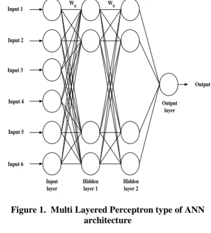
An ANN is interconnections of elementary simple processing units called neurons. Multi layered Perceptron (MLP) model of ANN is shown in figure 1. It consists of one input layer, one or more hidden layers and one output layer. Each layer consists of several neurons and these are connected to the neurons in the adjacent layers with different weights. Each neuron in the hidden layers and in the output layers receives signals from the previous layer neurons and produces the output signal by passing the summed signal through a sigmoid function. Thus the signal in ANN passes through input layer, hidden layers and produces output at the output layer.

Let us assume there are Psets of training data of which



i1,i2,...ip



is the input data set and



t1,t2,...tp



is the

(2)

The output of neuron

j

is defined as





 

_

x

_

e x f i O ij W where i O ij W i f j O        1 1 and i neuron the from Output j neuron and i neuron the between weight 1

The error at the kthoutput neuron is defined as follows





2

 

2

2 1 k O k t

E 



The updating of weights is done according to the equation given below

 

3

ij W j O j O E ij W E ij W             

Specifically, we define the error signal as

 

4

j O E j      

The generalized back propagation rule can be the following

 

   

 

neuron output the of one not is j f 1 neuron output the of one is j if 1 gain adaption where 5 i jk W k k j O j O j j O j O j O t j i O j ij W           



The convergence characteristics can be improved by introducing a momentum term with a momentum gain



to equation (5)

 

index iteration the represents n where 6

1 _jO_j W_ij n

n ij

W    

  

Once the neural network is trained it produces very fast output for a given validation data. It requires only a few arithmetic calculations of sigmoid function. To evaluate the accuracy of the neural network approach in forecasting electricity demands. This accuracy is computed in function of the actual market demands that occurred. The mean absolute percentage error MAPE criterion is applied

.

Input 1 Output Input layer Hidden layer 1 Hidden layer 2 Output layer Input 2 Input 3 Input 4 Input 5 Input 6

[image:2.595.321.528.77.306.2]

Wij Wij

Figure 1. Multi Layered Perceptron type of ANN architecture

 

     N t k t k O k t N MAPE

1 100 7

1

3. IMPLEMANTATION

Hourly demand data is collected from PJM electricity markets which is available in the website. The data for the month January 2014 has been used as Input to train the ANN for forecasting the PJM electricity demand. The original demand series is decomposed into two intrinsic modes with different scales. First one is based on the membership of an hour to classic demand forecasting model and another one is correlation dependent demand forecasting model. The details of divisions are described as follows.

3.1. Classic Demand Forecasting Model

A simpler subdivision in only two time blocks identifying off peak hours and peak hours has also been proposed. The data said is plotted as shown in fig. 2. The figure reveals that the hours 1 to 17 and 24 have the similar type of demand and the rest of the hours have similar type of demand. Depending on this observation the total 24 hours are divided into two time blocks and called as off peak hours and peak hours respectively. ANNs are trained separately to forecast the demand in off peak hours and peak hours. A slight difference exists in comparison with the classic F1 and F2 of the PJM Electricity Market. Inputs to the ANNs are past loads i.e. Ld-1 and Ld-7 and theoutputof the ANN is the load forecast for a given day d as shown in table 2.

3.2. Correlation Demand Forecasting

Model

(3)

[image:3.595.54.293.83.198.2]

Figure 2. Shows the demand curve for the month of January

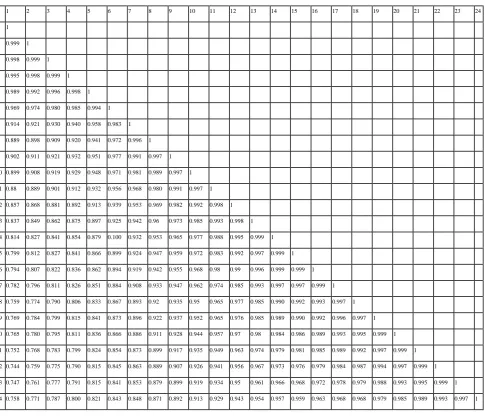
A correlation matrix has been computed, as shown in table 1, analyzing the available time series data on the PJM electricity

demands, over the month of January 2014. By means of this correlation matrix a number of classes of hours, in the remainder group of hours have been identified, in order to demonstrate how the demand forecast may be improved in terms of smaller error percentage, in comparison with the classic demand forecast on an hourly basis. Each group of hours has been identified by grouping together all the hours with a high correlation coefficient, thus yielding a number of groups which is higher than the ordinary groups of hours used within most of the electricity markets. This greater number of groups should then likely provide a more satisfactory result in terms of forecasting error, since each group contains a smaller number of hours, thus of uncertain variables to be treated separately. The 24 hours are grouped depending on the correlation coefficient greater than 0.99. According to this rule, seven groups have been established in total, and are shown in table 2

Table 1. Correlation matrix for the month of January 2014 of PJM electricity markets on hourly basis

1 2 3 4 5 6 7 8 9 10 11 12 13 14 15 16 17 18 19 20 21 22 23 24 1 1

2 0.999 1 3 0.998 0.999 1 4 0.995 0.998 0.999 1 5 0.989 0.992 0.996 0.998 1 6 0.969 0.974 0.980 0.985 0.994 1 7 0.914 0.921 0.930 0.940 0.958 0.983 1 8 0.889 0.898 0.909 0.920 0.941 0.972 0.996 1 9 0.902 0.911 0.921 0.932 0.951 0.977 0.991 0.997 1 10 0.899 0.908 0.919 0.929 0.948 0.971 0.981 0.989 0.997 1 11 0.88 0.889 0.901 0.912 0.932 0.956 0.968 0.980 0.991 0.997 1 12 0.857 0.868 0.881 0.892 0.913 0.939 0.953 0.969 0.982 0.992 0.998 1 13 0.837 0.849 0.862 0.875 0.897 0.925 0.942 0.96 0.973 0.985 0.993 0.998 1 14 0.814 0.827 0.841 0.854 0.879 0.100 0.932 0.953 0.965 0.977 0.988 0.995 0.999 1 15 0.799 0.812 0.827 0.841 0.866 0.899 0.924 0.947 0.959 0.972 0.983 0.992 0.997 0.999 1 16 0.794 0.807 0.822 0.836 0.862 0.894 0.919 0.942 0.955 0.968 0.98 0.99 0.996 0.999 0.999 1 17 0.782 0.796 0.811 0.826 0.851 0.884 0.908 0.933 0.947 0.962 0.974 0.985 0.993 0.997 0.997 0.999 1 18 0.759 0.774 0.790 0.806 0.833 0.867 0.893 0.92 0.935 0.95 0.965 0.977 0.985 0.990 0.992 0.993 0.997 1 19 0.769 0.784 0.799 0.815 0.841 0.873 0.896 0.922 0.937 0.952 0.965 0.976 0.985 0.989 0.990 0.992 0.996 0.997 1 20 0.765 0.780 0.795 0.811 0.836 0.866 0.886 0.911 0.928 0.944 0.957 0.97 0.98 0.984 0.986 0.989 0.993 0.995 0.999 1 21 0.752 0.768 0.783 0.799 0.824 0.854 0.873 0.899 0.917 0.935 0.949 0.963 0.974 0.979 0.981 0.985 0.989 0.992 0.997 0.999 1 22 0.744 0.759 0.775 0.790 0.815 0.845 0.863 0.889 0.907 0.926 0.941 0.956 0.967 0.973 0.976 0.979 0.984 0.987 0.994 0.997 0.999 1 23 0.747 0.761 0.777 0.791 0.815 0.841 0.853 0.879 0.899 0.919 0.934 0.95 0.961 0.966 0.968 0.972 0.978 0.979 0.988 0.993 0.995 0.999 1 24 0.758 0.771 0.787 0.800 0.821 0.843 0.848 0.871 0.892 0.913 0.929 0.943 0.954 0.957 0.959 0.963 0.968 0.968 0.979 0.985 0.989 0.993 0.997 1

0 20000 40000 60000 80000 100000 120000 140000 160000

1 ₂₃ ₄₅ ₆₇ ₈₉

111 133 155 177 199 221 243 265 287 309 331 353 375 397 419 441 463 485 507 529 551 573 595 617 639 661 683 705 727

De

m

an

d

(

M

w

)

Hours

[image:3.595.58.544.277.693.2]

(4)

[image:4.595.65.528.94.318.2]

Table 2. Different grouping of based on Classic demand forecasting model and Correlation demand forecasting model and their respective ANN structures

Models

No. of time Blocks

4. RESULTS

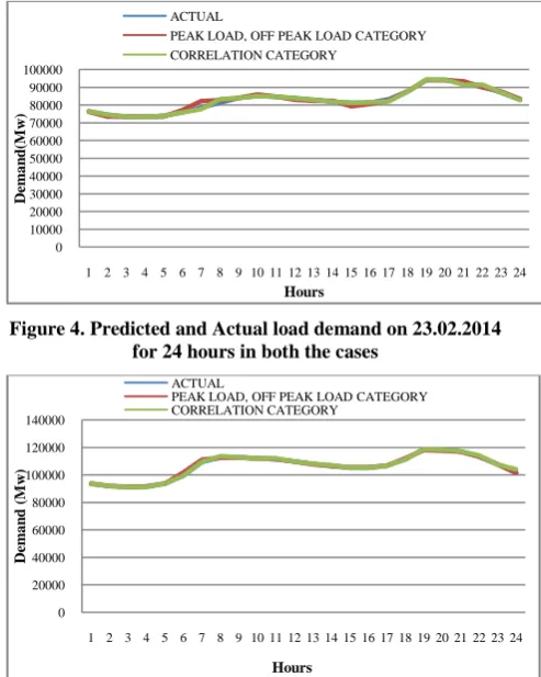
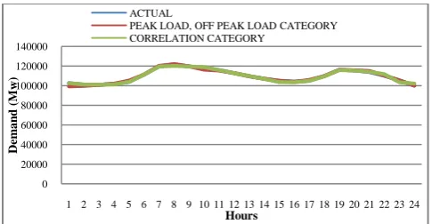
The proposed neural network approach is applied to forecast the electricity demands by using the two proposed models for three sample days in the PJM electricity markets. For testing the proposed ANNs MAPE for different cases are evaluated. In particular, February 23rd, 26th and 28th of the year 2014 which are weekly end day, weekly off day and weekly working day are assumed as the next days of which demand must be forecasted.

4.1. First Case

Table 2 describes different types of grouping of hours and required number of ANNs for demand forecasting. According to this model the forecasted day is divided into 2 groups namely peak load hours and off peak load hours. The demands for the peak load hours constitute of 6 hours of the day and off peak load hours constitute remaining 18 hours of the day, are forecasted separately. The days considered are outside the observation period used for training of ANNs. Here two ANNs are required for forecasting the demand for 24 hours of the prescribed days. A multi layered feed forward neural network which has 36 input neurons, 18 output neurons is implemented for forecasting demand of the off peak load hours. The first 18 neurons in the input layer corresponds to the 18 demands of previous day (relatively the day ahead) and the rest 18 neurons corresponds to 18 demands of the same day of the previous week. Similar distribution in input neurons regarding the previous day and same day of previous week are continued for every ANN through the rest of the paper. Further, the second neural network has 12 input neurons, 6 output neurons for demand forecasting of the peak load hours. Here also 6 input neurons belong to previous day and rest 6 input neurons belongs to same day of the previous week. The details of number of neurons in input layer and output layer are given in table 2. The structure of ANN showing input neurons and output neurons briefly is presented in the fig 2. After a good degree of training reaches, ANN is tested with unknown data and results are presented in figures 4, 5 & 6. The MAPE for the three prescribed days is presented in the table 3. The results show that there is good compromise between the actual values and predicted values along with minimum MAPEs. The results also reveal that the error produced by the proposed model is very low as compared to other conventional methods.

4.2. Second Case

[image:4.595.69.528.96.319.2]

Collected hourly demand data for the month January 2014 is used in establishing the correlation matrix for the identification of similarity in demand. Based on the correlation coefficient 7 group of hours are formed and used for training the ANN. The grouping of hours is represented in the table 2, According to this 7 different ANNs are trained to forecast the hourly demand on the prescribed days of interest.

Figure 4. Predicted and Actual load demand on 23.02.2014 for 24 hours in both the cases

Figure 5 Predicted and Actual load demand on 26.02.2014 for 24 hours in both the cases

0 10000 20000 30000 40000 50000 60000 70000 80000 90000 100000

1 2 3 4 5 6 7 8 9 10 11 12 13 14 15 16 17 18 19 20 21 22 23 24

De

m

an

d

(M

w

)

Hours ACTUAL

PEAK LOAD, OFF PEAK LOAD CATEGORY CORRELATION CATEGORY

0 20000 40000 60000 80000 100000 120000 140000

1 2 3 4 5 6 7 8 9 10 11 12 13 14 15 16 17 18 19 20 21 22 23 24

De

m

an

d

(

M

w

)

Hours ACTUAL

[image:4.595.312.560.403.541.2] [image:4.595.310.557.404.713.2]

(5)

[image:5.595.54.297.70.196.2]

Figure 6. Predicted and Actual load demand on 28.02.2014 for 24 hours in both the cases

Table 3. Comparison of MAPEs evaluated through different cases

Forecasted day

%MAPE based on Classical Demand forecasting model

%MAPE based on Correlation Demand

Forecasting Model 23.02.2014 0.8828 0.3426 26.02.2014 0.3442 0.2187 28.02.2014 0.4564 0.4483

5. CONCLUSION

This paper proposes Artificial Neural Network based hourly a day ahead demand forecasting model for PJM electricity markets. The demand forecasting is done based on classic demand forecasting model and correlation demand forecasting model. The day to be forecasted is divided into 7 groups of hours depending upon correlation coefficient. Similarly depending upon classic demand forecasting model the day to be forecasted is divided into peak load hours and off peak load hours. The performances of the ANNs are evaluated by calculating the MAPE in both the cases. The input data used as training data for ANN is the previous day data and same day of previous week data. The results explore that correlation based demand forecasting is best and suitable for PJM electricity markets than the classic demand forecasting model. The results conclude that the good quality of training data used for the ANNs improve the forecasting electricity demand. The MAPE evaluated through the proposed models are very low as compared to other conventional models. The proposed approach represents a useful method to forecast next-day electricity demands in the bidding process of energy market operators.

6. REFERENCES

[1] Tomonobu Senjyu, Hitoshi Takara, Katsumi Uezato, and Toshihisa Funabashi, “One hour-ahead load forecasting using neural network”, IEEE Trans. Power Systems, vol. 17, no. 1, Feb. 2002.

[2] T. Haida, and S. Muto, “Regression based peak load forecasting using a transformation technique,” IEEE Trans. Power Systems, vol. 9, pp.1788–1794, Nov. 1994. [3] A.G.Baklrtzis, V.Petrldis, S.J.Klartzis, M.C.Alexiadls,

A.H.Malssis, “A neural network short term load forecasting model for the greek power system”, IEEE Trans. Power Systems, vol.11, no. 2, May 1996.

[4] Kim K, Youn HS, Kang YC. Short-term load forecasting for special days in anomalous load conditions using neural

networks and fuzzy inference method. IEEE Trans. Power Systems vol. 15, pp. 559–65, 2000.

[5] Charytoniuk W, Chen MS. Very short-term load forecasting using artiﬁcial neural networks. IEEE Trans. Power Systems, vol.15, pp. 263–8, 2000.

[6] Hippert HS, Pedreira CE, Souza RC. Neural networks for short-term load forecasting: a review and evaluation.

IEEE Trans. Power Systems, vol. 16, pp. 44–55, 2001. [7] A.S.Dhdashti,J.R.Tudor,andM.C.Smith, “Forecasting of

Hourly Load By Pattern Recognition: A Deterministic Approach,” IEEE Trans. Power Apparatus and Systems, vol. 101, No. 9, pp. 3290–3294, Sept. 1982.

[8] J. Toyada, M. Chen, and Y. Inoue, “An Application of State Estimation to Short-Term Load Forecasting, I and II,” IEEE Trans. Power Systems, vol. 89, pp. 1678–1688, Sept. 1970.

[9] Charytoniuk W, Chen MS, Olinda PV. Nonparametric regression based short-term load forecasting. IEEE Trans. Power Systems, vol. 13, pp. 725–30, 1998.

[10]Kun-Long Ho, Yuan-Yih Hsu, Chih-Chien Liang, Tsau-Shin Lai “Short-Term Load Forecasting of Taiwan Power System Using A Knowledge-Based Expert Systems”,

IEEE Trans. Power Systems, Vol. 5, No. 4, Nov 1990. [11]Papalexopoulos AD, Hao S, Peng T. An implementation

of a neural network based forecasting model for the EMS.

IEEE Trans. Power Systems, vol. 91, pp. 956–62, 1994 [12]Henrique Steinherz Hippert, Carlos Eduardo Pedreira, and

ReinaldoCastro Souza. “Neural Networks for Short-Term Load Forecasting: AReview and Evaluation”. IEEE Transactions on Power Systems, Vol. 16, No. 1, Feb. 2001.

[13]S. Rahman and R. Bhatnagar, “An Expert System Based Algorithm for Short-Term Load Forecast,” IEEE Trans. Power Systems, vol. 3, No. 2, May 1988, pp. 392–399. [14]S. E. Papadakis, “A Novel Approach to Short-Term Load

Forecasting Using Fuzzy Neural Network,” IEEE Trans. Power Systems, vol. 13, No. 2, May 1998, pp. 480–492. [15]P. K. Dash, H. P. Satpathy, A. C. Liew, and S. Rahman,

“A Real-time Short-Term Load Forecasting System Using Functional Link Network,” IEEE Trans. Power Systems, vol. 12, No. 2, May 1997, pp. 675–680

[16]C.N.Lu,H.T.Wu,andS.Vemuri,“Neural Network Based Short Term Load Forecasting,” IEEE Trans. Power Systems, vol. 8, No. 1, Feb. 1993, pp. 337–342.

[17]J. Vermaak, “Recurrent Neural Networks for Short-Term Load Forecasting,” IEEE Trans. Power Systems, vol. 13, No. 1, pp. 126–132, Feb. 1998.

[18]D. Papalexopoulos, S. Hao, and T. M. Peng, “An Implementation of a Neural Network Based Load Forecasting Model for the EMS,” IEEE Trans. Power Systems, vol. 9, no. 4, pp. 1956–1962, Nov. 1994. [19]T. Zheng, A. A. Girgis, and E. B. Makram, “A Hybrid

Wavelet Kalman Filter Method for Load Forecasting,” Electric Power Systems Research, vol. 54, No. 1, pp. 11– 17, April 2000,.

[20]Chow TWS, Leung CT. Nonlinear autoregressive integrated neural network model for short-term load

0 20000 40000 60000 80000 100000 120000 140000

1 2 3 4 5 6 7 8 9 10 11 12 13 14 15 16 17 18 19 20 21 22 23 24

De

m

an

d

(

M

w

)

Hours ACTUAL

(6)

forecasting. IEEE Proc. Gene. Trans. Distrib., vol. 14, pp. 3500–6, 1996.

[21]Lamedica R, Prudenzi A, Sforna M, Caciotta M, Cencellli VO, “A neural network based technique for short-term forecasting of anomalous load periods,” IEEE Trans. Power Systems, vol. 11, pp. 1749–55, 1996.

[22]AlFuhaid AS, El-Sayed MA, Mahmoud MS. Cascaded artiﬁcial neural networks for short-term load forecasting.

IEEE Trans. Power Systems, vol. 121, pp. 524–9, 1997.

[23]Lu CN, Vemuri S, “Neural network based short term load forecasting,” IEEE Trans. Power Systems, vol.8, pp. 336– 42, 1993.