Journal of Chemical and Pharmaceutical Research, 2014, 6(3):131-140
Research Article
CODEN(USA) : JCPRC5
ISSN : 0975-7384
Research and application of the combined model of principal component
analysis and neural network based on SPSS
Jianhui Wu
1*, Hongbo Shao
2, Yu Su
1, Zhengjun Guo
1, Sufeng Yin
1, Houjun Xu
1, Bo Hu
1,
Liqun Yu
1and Guoli Wang
1*
1Hebei Province Key Laboratory of Occupational Health and safety for Coal Industry, Division of Epidemiology
and Health Statistics, Hebei United University, Tang Shan, China
2College of Science, Agricultural University of Hebei, Baoding, China 3College of science, Hebei United University, Tang Shan, China
_____________________________________________________________________________________________
ABSTRACT
BP neural network is widely used in many fields, this method shows a lot of shortcomings. In this article, the principle component analysis and BP neural network are combined together to establish a combined prediction model based on SPSS. Firstly, we should use principle component analysis to reduce the dimension of the variables and eliminate the colinearity among the variables. According to the selected principle components, BP neural network model will be built. By comparing with the result of single BP neural network model, the fitting degree (R2=0.9018) of the combined model is better than that (R2=0.8359) of the single one. After comparing the average
differences of two models, we have found that the prediction ability (MSE=0.16) of the combined model is better than that (MSE=0.22) of the single model, which shows that the multicolinearity of the resolution factors. It can reduce the data dimension, optimize the structure of neural network, and quicken the speed of the network training and study. The function of the established combined model is good, and it had good plasticity in SPSS, which can be promoted in the prediction field.
Keywords:Principle Component Analysis; BP neural network; Prediction; Combination model; SPSS
_____________________________________________________________________________________________
INTRODUCTION
theory of reducing dimension to find some independent comprehensive indexes to summarize the original indexes information [4]. Meanwhile, it also can solve the colinearity. If we combine it with BP neural network to form a conbined prediction model, whether this model can offset the shortcomings of the data structure and influential factors, improve PB neural network model building process, make the result more objective and scientific is worth discussing [2]. In this article, we discuss the combined prediction model of principle component analysis and BP neural network and plan to provide a new way to implement the prediction research.
THEORY OF COMBINED MODEL
Establishment of Single BP Neural Network Model
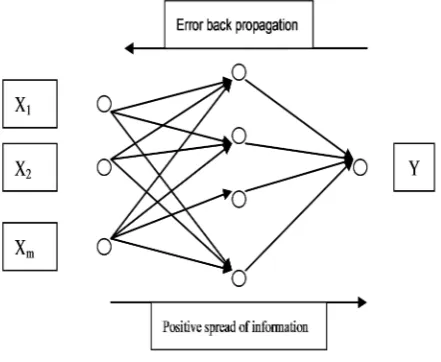
[image:2.595.198.419.206.387.2]One typical BP neural network is made up of input layer, output layer and hidden layer. And the hidden layer may be one layered or multiple layered.
Fig. 1 The structure of BP neural network
The basic principle of BP neural network
BP (Back Propagation) neural network is the study process of error back propagation algorithm which is made up of information forward propagation and error back propagation. The neurons in input layer are responsible for receiving the input information from outside and then deliver the information to the neurons in the hidden layer. The hidden layer is the inner information processing layer which is responsible for information conversion [1]. The information delivered to the output layer from hidden layer can finish the forward propagation process once after the further processing. The information processing result will be output by the output layer. When the signals are forward propagated, the weight of the network will not be changed. The output of the neurons in each layer only affects the status of the neurons in the next layer. When the actual output does not correspond to the prediction, the error back propagation will be started. The errors will go through the output layer, correct the values of weight according to the gradient descent and back propagate to the hidden layer and output layer. In the process of the error back propagation, the values of weight are continuously corrected and adjusted, shortening the distance between the practical output and the desired output. This is the network output training process. It will last till the errors output from the network are reduced to the acceptable level or the set training times are reached [6]. Compared with the traditional statistic method, BP neural network has no hypothesis requirement on the data. The strong function approximation ability makes the network is better than the traditional statistic method [7].
The steps of BP neural network modeling A. Data normalization
In practice, by normalizing the output and input variables, the network training will be more effective [8] . The training speed of the network and the function of the network will be improved. The detailed normalization method will be diversified according to the data, which generally are orthonormality, change of scale and standardization. The change of scale means that after being added or deducted a constant the changed variable will be multiplied or divided by a constant. It mainly is used to change the unit of the data. The orthonormality will implement the normal conversion with the typical value 0 and the standard deviation 1 or normalize it within the scope of [-1, 1]. Standardization means we directly compress the data within the scope of [0, 1]. The formulas are as below,
std mean x
S i i
2 / )) min( ) (max(
2 / )) min( ) (max(
x x
x x
x S i
i
(2)
) min( ) max(
) min(
x x
x x
S i
i
(3)
When classifying the variables, we can adjust formulas of the orthonormality and standardization. To continue the variables, we can use orthonormality and standardization formulas. Because the input and output variables are of positive values, the values of selected variables by the standardization formula are within the scope of [0,1] considering the selection rules of transmission functions and data distribution. After the network simulation, the anti-normalization is used to convert the simulation result to original data.
B. The selection of the transfer function
BP neural network needs differentiable non-linear functions, such as S-functions: logarithm S-function and hyperbolic tangent function. We don’t have definite standard of choosing S-functions. Generally speaking, if the values of input variables are more than 0, we’d better use logarithm S-function. If the values of the output variables are less than 0, we’d better use hyperbolic tangent function. For the neurons using S-functions, the input data should be normalized to [0, 1] or [l, 1]. So the saturation region of the function and the slow speed of the network convergence are avoided. Because the variable values are all more than 0 in this research, we use S-function which is logsig function.
C. The partition of data sets
The partition of data sets is very important. After the study of the training set, we establish a model with good promotion function. The training sets should be well distributed, which are good representatives of the sample set. The training set and verification set are applied in the network training and model prediction. The test set is used to trace the mistakes in the training to avoid over fitting [9].
We adopt different strategies to improve the promotion abilities of the network. They have different requirements on the data set. If we use early stop strategy, the data sets should be divided into training sets (60%), verifying sets (20%) and test sets (20%). If we use Bayes rules BP algorithm, the data sets will be divided into training sets (80%) and test sets (20%).
D. Initialized weights and thresholds
When initializing the network, to initialize the weights and threshold correctly is very important [10]. If the initialization is not proper, the training time may be longer and even the network can not be converged. If the initial value is large, the weighted value may be within the saturation region of the transfer function which results in the small descent gradient. It will lead to the stop of the training of the network. Generally, we hope that the initialized weighted values of the neurons are close to zero so that the weights of the neurons can be adjusted in the most sensitive region of change in the S-function. Therefore, the initial values of weight and threshold are randomly selected within [-1, 1].
E. The speed of initialized learning
The learning speed can determine the changes of the weights in the process of network training. When the learning speed is slow, the change margin of the weights is small, which will lead to the slow network training and difficult convergence of the network. While the learning speed is too fast, the system will be unsteady and the weight value and error function will be different, which means the sum of squared errors of the network function can not reach a suitable value. At present, the adopted BP algorithm is not a standard one which is an improved BP algorithm, such as LM algorithm, conjugate gradient algorithm and etc. These algorithms can quicken the speed of network convergence by improving the standard BP algorithm [12].
F. The evaluation indexes of network function
For the approximation of the function, the network function evaluation can be influenced by the goodness of fit between the value of fitting of the model and the measured value. It also can be reflect by sum of squared errors (SSE), coefficient of determination (R2), adjusted coefficient of determination (adjusted R2), root mean square error
(RMSE), mean square error (MSE) and other indexes. In this article, the coefficient of determination (R2) is selected
to evaluate the network function [11].
G. The selection of training algorithm
algorithm (regarded as trainscg in MATALB) of Bayes rules is one method to increase the prediction accuracy of the network. Mutative scale conjugate gradient algorithm (regarded as trainbr in MATLAB) is comparatively good which performs well in prediction and function approximation. Quasi-Newton algorithm (regarded as trainoss in MATLAB) is faster in the convergence than the mutative scale conjugate gradient algorithm [13].
H. The set of number of layers of the neural network and neurons in each layer
The determination of number of layers in the network: one 3-layer neural network can implement the approximation of any nonlinear function with the desired accuracy. Generally, one-layer or two-layer hidden layer is enough to solve the practical problems. The adding of the layers will make the network complicated, which will influence the convergence speed of the network [14].
The determination of the number of neurons of each layer: the number of the neurons in the input and output layers should be determined according to the practice. They are just like the independent variables and dependent variables. At present, there is no definite formula to determine the number of the neurons in the hidden layer. If we calculate by the experienced formula, the result may be quite different. When using trial-and-error method, m refers to the number of neurons in input layer; n refers to the number of the neurons in the hidden layer; we have n=log2m. If the
convergence is not ideal, the number of the neurons will be added. If the errors can’t be reduced and the convergence speed is slow, we should consider the stop the adding; or we can suppose n=2m+1 according to Komlogorov theorem [15].
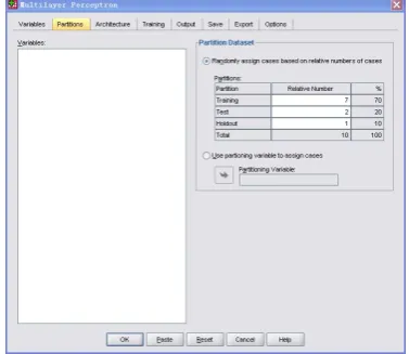
The implementation process of SPSS
[image:4.595.212.401.343.533.2]Using SPSS17.0 software for the following operation, Analyze→Neural Networks→Multilayer Perceptron→ Choose the dependent variable→Choose the independent variable, which is shown as Fig.2.
Fig. 2 The variables TAB
Distribution of training samples and testing samples and support the proportion of samples were 70%, 20% and 10%, respectively.
[image:4.595.211.400.585.748.2]Choose custom system structure, the number of hidden layers on the "two layer", choose "hyperbolic tangent" hidden layer activation function, hidden layer unit number to choose "automatic calculation", choose "hyperbolic tangent" output layer activation function.
Fig. 4 The architecture TAB
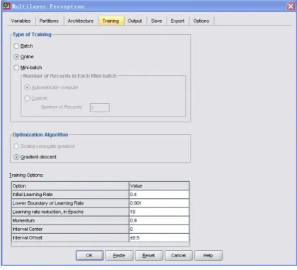
Choose "online" training types, optimization algorithm is used to select the "gradient", training options vector of initial vector, the vector of lower limit, the schedule to reduce, kinetic energy, central point and interval between offset using the default values.
Fig. 5 The training TAB
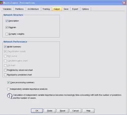
[image:5.595.201.411.381.571.2]Fig. 6 The output TAB
The principal component analysis
The basic principle of principal component analysis
Suppose there are p indexes X1,X2,…,Xp.We should find the independent comprehensive indexes Z1, Z2, Zp,
which can summarize the information of p indexes. From the perspective of mathematics, we should find a group of constants ai1, ai2…, aip(i=1, 2…, p) and linear combine p indexes.
p pp p p p p p p p X a X a X a Z X a X a X a Z X a X a X a Z 2 2 1 1 2 2 12 1 11 2 1 2 12 1 11 1 (4)
In order to summarize the main information of p original indexes X1, X2…, Xp, we introduce the following matrix,
P Z Z Z Z 2 1 ' ' 2 ' 1 12 1 2 22 21 1 12 11 p pp p p p p a a a a a a a a a a a a A p X X X X 2 1
Formula (1-1) can be illustrated as
Z=AX (5) Or X a Z X a Z X a Z p p ' ' 2 2 ' 1 1 (6)
If Z a'X
1
1 satisfies 1 1 ' 1a
a and ( ) { ( ' )} 1 1 1 ' 1 X a Var Max Z Var a a
, Z1is the first principal component of original indexes
X1, X2…, Xp. When Zi≠Zj, Ziand Zjhave no relation and Z1is the maximum variance of all the linear combinations
of X1, X2…, Xp. And Z2ranks the second. The rest may be deduced by analogy.
2.2.2 The basic steps of principal component analysis
j j ij ij
s
x
x
z
(7)In the formula, j xij
n x n i
1 1 ] ) ( 1 1 [ 2 1 j ijj x x
n s n i
i=1, 2…, n j=1, 2…, p
After the transmission, the typical value is zero and the variance is one.
The reason of orthonormality of the original data: when solving the principal component by the related coefficient matrix R, we usually pay more attention to the larger variable of variance 2
j
, which means that it will be influenced by the measurement scale of the variables and sometimes we will get unreasonable result. In order to illustrate the connotation of the principal component more objectively, we must normalize the original data and eliminate the impacts of the unit of measurements and order of magnitude.
2) Solving the related matrix R of indexes
The variable related matrix R is the starting point of principal component analysis. The measurement formula is
k j i
s
x
x
s
x
x
n
r
n ij i ik ki k
)
(
)
(
11
1
(8)Or ik
Z
ijZ
jkn
r
n i
11
1
(9)And Rii=1 rik=rkj
3) Solving the latent root, eigenvector and contribution rate of matrix R
The secular equation of R is
R
=0;
g (g=1, 2…, P) is the latent root of the equation and the variance of theprincipal component Z; the amount shows the information ability of the principal component comprehensive original indexes. We use L to represent the dimensional real vector. The vector Lg obtained from equation
g
R
L
g=0 is the corresponding eigenvector of the latent root
g , which is the sub-vector coefficients in thecoordinate system of standardized vector
jpj Z Z i j Z Z 1
. ag=
g / gp
g
1
shows the each principal component can
reflect the information amount of the original variable. That is the variance contribution rate.
4) The selection of amount of the principal components
Theoretically speaking, the maximum number of the principal components equals to the number of the original variables, which can reflect all the information provided by the all the original indexes. Because the aim of the analysis is to use less comprehensive indexes to reflect the main information of all the original indexes, the total number of the principal components is less than the number of the original indexes. There are a lot of principles in determining the number of components, which are shown below,
1 Cumulative contribution rate guideline
How many principal components will be kept is determined by the percentage of the cumulative variance in the sum of the variances (cumulative contribution rate). It shows the how much information the previous principal components have. Generally when the cumulative contribution rate of k principal components reaches 80%, k principal components[16]should be kept.
②Latent root guideline
First the typical value of latent root λgshould be calculated. Select k sub-vectors which are λg> as principal
3 The final determination of principal components
The principal components got from cumulative contribution rate are always a lot, while the components got from latent root method are rare. So we will consider the combination of cumulative contribution rate and latent root to determine the final principal components and considering the professional significance of variables to determine if necessary.
The establishment of the combination model of principal components analysis and BP neural network
First we should implement the principal components analysis to all the prediction factors and save the selected principal component score matrix.
The comparison of the fitting effects of the model
Select single BP model and combination model and use the prediction value and the errors of the truth value by t test to evaluate the effect of the model.
APPLICATION EXAMPLE Object of study
The objects of the study are coal worker’s pneumoconiosis patients from 3 branch ores in a mining industry group since 1988. The data is from the occupational disease returns, occupational disease diagnoses certificates and physical examination forms. According to the diagnose standard and study object selection standard, we have effective 599 samples.
The selection of influencing factors
We select six factors which will influence pneumoconiosis according to the report in the literature, such as type of work, length of being exposed to the dust, classification of ores, date of birth, time of starting to be exposed to the dust, and age of starting to be exposed to the dust.
Result of single BP neural network model
[image:8.595.154.461.459.536.2]Using SPSS17.0 we establish BP neural network model and parameters. The input variables are type of work, length of being exposed to the dust, classification of ores, date of birth, time of starting to be exposed to the dust, and the output variable is the age of starting to be exposed to the dust. By self set and automatic debugging of the software, the main parameters of the optimal BP neural network model are shown in Table 1
Table 1: Main parameters of BP neural network model
Parameters of network structure Parameters of network training
Number of hidden layers: 1 Number of iterations when training stops: 11 Number of neurons in hidden layer: 9 Learning speed: 0.1
Number of neurons in input layer: 6 Performance function: SSE
Number of neurons in output layer: 1 Training set when training stops SSE=0.852 Activation function in hidden layer: Sigmoid Test set when training stops SSE=0.219 Activation function in output layer: Sigmoid Training set R2=0.8132
Training algorithm: Gradient descent method Test set R2=0.8359
The result of principal components analysis
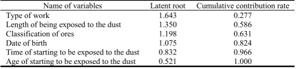
We implemented the principal component analysis to the influencing factors of length of being exposed to the dust. The result is shown in Table 2.
If the absolute value of the factor loadings is more, the correlation with the principal components is more. After the analysis of the twiddle factor loading matrix, we find that the first principal component mainly represents the main information of length of being exposed to the dust, time of starting to be exposed to the dust, and age of starting to be exposed to the dust; the second principal component represents the main information of type of work; the third one mainly represents the information of classification of ores; and the fourth one represents the information of the date of birth.
Table 2: Result of principal component analysis
Name of variables Latent root Cumulative contribution rate Type of work 1.643 0.277
[image:8.595.159.454.679.748.2]Select four principal components according to latent root and cumulative contribution rate; based on the factor loading matrix, we can obtain the following equations of the principal components.
Z1=0.325X1+0.587X2+0.289X3+0.2915X4+0.481X5+0.463X6 Z2=0.586X1+0.355X2+0.361X3+0.044X4+0.219X5+0.238X6 Z3=0.375X1+0.210X2+0.595X3+0.314X4+0.141X5+0.155X6 Z4=0.292X1+0.147X2+0.248X3+0.485X4+0.235X5+0.199X6
3.5. The modeling of BP neural network based on principal component analysis
[image:9.595.149.464.240.319.2]Taking the selected principal component score matrix as the input variable and the total hospital charges as the output variables, we establish a model of BP neural network based on principal components. The result of the model is shown in Table 3.
Table 3: Main parameters of BP neural network combination model based on principal components
Network structure parameters Network training parameters
Number of hidden layers: 1 Number of iterations when training stops: 10 Number of neurons in hidden layer: 8 Learning speed:0.1
Number of neurons in input layer: 4 Performance function: SSE
Number of neurons in output layer: 1 Training set when training stops SSE=0.459 Activation function in hidden layer: Sigmoid Test set when training stops SSE=0.162 Activation function output layer: Sigmoid Training set R2=0.8672
Training algorithm: gradient descent method Test set R2=0.9018
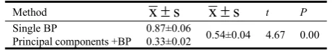
The test of model effects
Compare the values of residual errors of the two methods and the result are shown in Table 4.
Table 4: The effect comparison between single model and combination model (n=599)
Method
x
s
x
s
t PSingle BP 0.87±0.06 0.54±0.04 4.67 0.00 Principal components +BP 0.33±0.02
From the pair t test of two groups of residual errors values, the residual error value of single BP neural network is 0.87; the residual error value of BP neural network based on principal components is 0.33, t=4.67,P<0.05. The result shows that the two methods are different. Through comparing the values of residual errors, we can see that the prediction ability of BP neural network based on principal components is better.
CONCLUSION
In this research, we combine principal component analysis and BP neural network to establish a combination prediction model. The performance and prediction effect are both better than those of single BP neural network model, which means that principal component analysis can solve the multicolinearity among the factors, reduce the dimension of the data, optimize the neural network structure and quicken the training and learning speed of the network. This model does great help in prediction of pneumoconiosis and can be promoted applied in the prediction field.
Acknowledgements
This work is supported by Hebei Science and Technology Funds (11276911D), program of Tangshan Science and Technology Research and Development (11150205A-3), the accented term of Health Department of Hebei Province (20120146).
REFERENCES
[1] Seott DF, Grayson RL, Metz EA,Occupation and Environmental Medicine, Vol. 46, No.12,2004, pp.1272-1277.
[2] Bartfay E, Mackillop WJ, Peter JL,Eur J Cancer Care (Engl), Vol.15, No. 2,2006, pp.115-124. [3] Duh MS, Walker A, Ayanian J Z,Am J Epidemiology, No. 14,2004, pp.464-471.
[4] W. Benhong, Q. Benedicte, K. Jocelyne, et al,Euphytica, No.132,2003, pp. 375-384.
[image:9.595.186.426.382.419.2][7] Suarthana E,Moons KG,Heederik D,et al.Occupation and Environmental Medicine,2007, Vol. 64, No.9, pp. 595- 601.
[8] TIAN Lu-jia, LIU Hong-bo, YANG Yong-li, et al,Chinese Journal of Industrial Medicine,2009,Vol. 22, No.2, pp.127-128.
[9] CHEN Yin-pin, FAN Hong-min, YUAN Ju-xiang, et al,Chinese Journal of Public Health,2009, Vol.25, No.5, pp.623-624.
[10] ZHU Da-qi, SHI Hui, “An introduction to artificial neural network and its application “,BeiJing: science press, 2006, pp.33.
[11] Huajuan Dai, “Study on the combination forecasting model and its application”, Chasha: Central South University,2007.
[12] Liuda Hu, “Non-linear Programming”,BeiJing: Higher Education Press,1990. [13] Donaldson,R.G, M.Kamstra,Journal of Forecasting,1996, No.15, pp.49-61.
[14] Simon HD Mamuya, Magne Bratveit, Yohana Mashalla, et al,A cross sectional study.BMC Public Health, 2007, No.7, pp.17-24.