Cadmium in the shallow groundwater of urban area: Spatial and statistical analysis

Journal of Chemical and Pharmaceutical Research, 2014, 6(6):556-561

Research Article

_{CODEN(USA) : JCPRC5}

ISSN : 0975-7384

Cadmium in the shallow groundwater of urban area:

Spatial and statistical analysis

Sun Linhua

School of Earth Science and Engineering, Suzhou University, Suzhou, Anhui, China

ABSTRACT

In this study, sixty-two shallow groundwater samples from the urban area in Suzhou, northern Anhui Province, China have been collected and analyzed for their cadmium concentrations, and then processed by either spatial analyses (spatial clustering) and statistical (box plot) for identifying the spatial and statistical outliers. The results indicate that fifteen samples have been identified as spatial outliers, whereas three samples have been identified as statistical outliers. Their mean±2σ concentration is then set as environmental baseline (0.035-1.062 ug/l). Moreover, based on the contour map of cadmium concentrations before and after outlier removing, one hotspot with high cadmium concentrations has been identified, which might be indication of anthropogenic contribution.

Key words: Cadmium, Environmental baseline, Shallow groundwater, Spatial outlier, Statistical outlier

____________________________________________________________________________________________

INTRODUCTION

The environmental background has attracted large number of studies because of its importance for environmental management. They include not only the environmental scientists [1, 2], but also the international and national organizations. Taking for instance, the environmental background as suggested by the Chinese Environmental Protection Administration [3] has long been used for the evaluation of local pollution degrees. However, these environmental background data might be meaningless because it was obtained in a national scale, rather than a local scale, which is considered to be different from area to area [4, 5]. Moreover, some environmental scientists suggest that a local environmental background, which should be obtained under the condition without any anthropogenic contribution, cannot be obtained because the whole world in nowadays has been affected by human activities. And therefore, the environmental baseline, a replacement of environmental background has been postulated for instead [6].

Therefore, a series of methods, including either statistical or non-statistical, have been carried out for solving the issue of local environmental baseline values. Among the statistical methods, the hypothesis of the normality or log-normality of concentration distribution, has long been used for determine the environmental baseline. For instance, the cumulative probability plot and Q-Q plot [7, 8], as well as the model based objective methods (including iterative 2σ technique and the calculated distribution function) [9, 10] have long been used for baseline studies. These studies revealed that it is more realistic to view geochemical baseline as a range of values rather than an absolute value.

outliers. It will be useful for the local groundwater management and protection.

EXPERIMENTAL SECTION

SITE DESCRIPTION AND SAMPLING:

Suzhou is surface water lacking city located in the northern Anhui Province, China because the annual rainfall is only 774 - 895 mm and most of them are concentrated mainly in the period May to September [12]. And therefore, the groundwater is important for the industrial, agricultural and domestic use in the area. An obvious phenomenon is that although most of the persons use centralized water supply in the urban area, more than 30% of the residences use water pumped from shallow wells (< 30 m). However, the environmental issues related to the shallow groundwater have not been well determined yet.

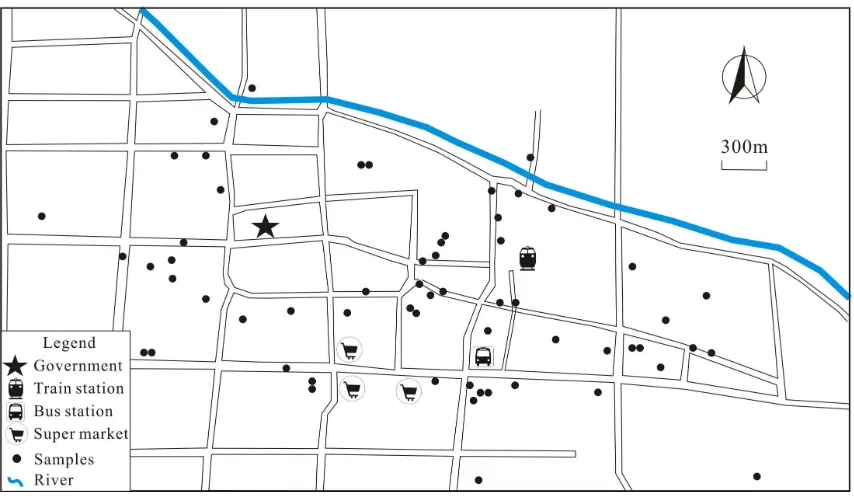
Fig. 1: Sample locations in the study area

And therefore, in this study, a total of sixty-two shallow groundwater samples have been collected from these wells in the urban area of the city during the period between September and October, 2013 (Fig. 1). All of the samples were firstly filtered by 0.45 µm pore-size membranes, and then immediately acidified to pH < 2 with HNO3 for preventing the precipitation and/or adsorption of elements by the bottle. Finally, the samples were sent for analysis within 24 hours in the Engineering and Technology Research Center of Coal Exploration in Anhui Province, China. The concentrations of cadmium were determined by Atomic absorption spectrometer with the coefficient of the calibration curve better than 0.99.

DATA ANALYSES:

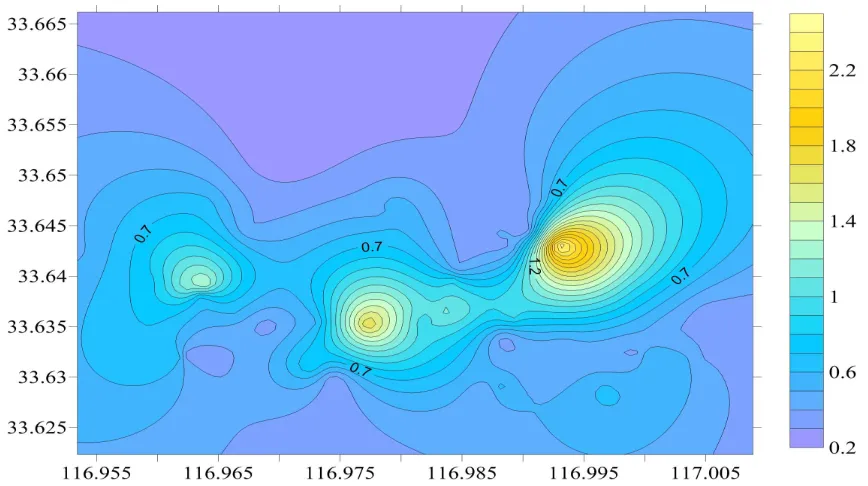
All of the concentrations were firstly processed by the software Mystat (version 12), and the minimum, maximum, mean, standard deviation, coefficient of variation, skewness and significant value of Anderson-darling normality test have been obtained. And then, the software Surfer (version 11) has been applied for producing the contour map of concentrations for identifying the spatial distribution characteristics.

Finally, the software GeoDa (version 1.4.6) has been applied for either statistical or spatial analysis, the detailed processes are as follows:

(1) Spatial cluster analysis, which names Univariate Local Moran’s I in the GeoDa software, has been applied for the dataset, and five categories (including not significant, high-high, low-low, low-high and high-low) can be obtained. The samples in high-high cluster were determined as hotspot samples, whereas samples in low-high and high-low clusters were selected as outliers. And then all of these samples were identified as spatial outliers.

calculation of the fences is listed below:

Lower fence: 25% percentile – 1.5×(75% percentile - 25% percentile).

Upper fence: 75% percentile + 1.5×(75% percentile - 25% percentile).

(3) After removing the statistical and spatial outliers, the mean±2σ [9] of the rest of the samples was then considered to be baseline values.

RESULTS AND DISCUSSION

CADMIUM CONCENTRATIONS:

The descriptive statistics of the cadmium concentrations (ug/l) are synthesized in Table 1. As can be seen from the table, the cadmium concentrations of the samples in this study range from 0.207 to 2.420 ug/l with mean and median values equal to 0.505 and 0.650 ug/l, respectively. In comparison with the quality standards for groundwater in China (µg/L, GB/T 14848-93), the samples in this study can be subdivided into two categories: most of the samples (fifty-two) are classified to be class II (≤ 1 ug/l), and ten samples are classified to be class III (≤ 10 ug/l). This result suggests that all of the samples in this study can meet the requirement for drinking, irrigation and industry directly based on their cadmium concentrations. Even in comparison with the WHO standard (3 ug/l) [13], all of the samples are suitable for drinking.

The spatial distribution of the cadmium concentrations in the shallow groundwater shows moderate coefficient of variation (0.593), implying that the cadmium in the shallow groundwater system might has not been dramatically affected by human activities, which is similar to the good quality of the groundwater. Moreover, as can be seen from the contour map of cadmium concentrations (Fig. 2), there are three areas of high cadmium concentrations (left, central and right of the map), which might be an indication of the anthropogenic effects.

It can also be obtained from Table 1 that the p-value of Anderson-Darling normality test is less than 0.05, implying that the cadmium concentrations of the samples in this study cannot pass the normality test, which might be a suggestion of the existence of anthropogenic contribution. However, it can get a higher p-value (0.031) after log-transformation, which might an indication of the lognormal distribution of cadmium concentrations (Table 1). And therefore, all of the data were then log-transformed before analyzes.

TABLE-1 Summary statistics of the whole dataset and those resulting from outlier removing

Whole1 _Whole2 _{Box plot}2 _{Spatial cluster}2 _Combine2

N of cases 62 62 62 50 47

N of outliers 0 0 0 12 15

Minimum 0.207 -1.573 -1.573 -1.573 -1.573

Maximum 2.420 0.884 0.884 0.884 0.064

Median 0.505 -0.684 -0.684 -0.751 -0.751

Mean 0.650 -0.562 -0.562 -0.635 -0.712

Standard deviation 0.386 0.494 0.494 0.476 0.369

Coefficient of variation 0.593 -0.879 -0.879 -0.749 -0.518

Skewness 2.185 0.603 0.603 0.916 0.188

p-value <0.01 0.031 0.031 0.018 0.15

Note: 1 and 2 mean before and after log-transformation, respectively. The unit for 1 is ug/l.

OUTLIER IDENTIFZICATION:

In this study, all of cadmium concentrations after log-transformation were firstly examined by box plot for identifying the statistical outliers. Based on the functions listed above, the lower and upper inner fences in this study were calculated to be -1.985 and 0.903 (log-ug/l), respectively, which equal to 0.010 and 7.998 ug/l, respectively. And this is no sample can be identified as outliers.

Relative to the statistical outliers, the samples with unusual values relative to their neighborhood are also considered to be outliers (spatial outlier) [14], and a series of methods have been applied. Among these methods, the Moran’s I is a commonly used indicator of spatial autocorrelation. There are two types of Moran’s I have been reported previously: one is the global Moran’s I, which is used to study the overall spatial autocorrelation, another one is LISA (local indicators of spatial association), which is applied to identify the degree of spatial autocorrelation in each specific location [15].

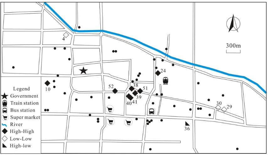
Based on the calculation of GeoDa, all of the samples in this study have been classified into two categories: not significant (50 samples) and significant (12 samples). Moreover, all of the significant samples can be classified into three secondary categories: eight, three and one samples are classified to be high-high (sample 10, 24, 38, 39, 40, 41, 51 and 52), low-low (sample 4, 29 and 30) and high-low (sample 36) clusters, respectively.

Fig. 3 Spatial outlier distribution

After these processes, the rest of the samples are only fifty, and then, the box plot has been applied for the rest of the samples and three samples (sample 23, 53 and 60) have been identified as statistical outliers.

BASELINE EVALUATION:

The synthesized data with and without outlier removing are listed in Table 1. Comparatively, based on the statistical method (box plot after log-transformation), no outlier has been identified. However, twelve samples have been identified after spatial analysis based on the data after log-transformation, which can be used for removing the spatial outlier samples. Because statistical method can only be used for removing the samples with extreme high values, and it is therefore inadequate to define the unique environmental baseline in a local scale without consideration the spatial variability simultaneously [14]. And therefore, the combination use of statistical and spatial analyses can get more reliable information.

As can be seen from the table, after outlier removing by spatial analysis, the rest of the samples give an mean concentration to be -0.635 (log-ug/l) and the p-value of lognormality test is 0.018, indicating that they cannot pass the lognormality test. However, after spatial and statistical outlier removing, the mean value of the rest of the samples is -0.712 (log-ug/l) and the p-value of lognormality test is 0.150, and the environmental baseline according to previous studies [9] is therefore established to be -1.450 – 0.026 (log-ug/l), which equals to 0.035 – 1.062 ug/l. This result is similar to the results obtained by using model based objective methods (iterative 2σ technique and the calculated distribution function) [9], the baseline values determined by the two kinds of methods are 0.2 – 0.7 and 0.2 – 0.8 ug/l, respectively.

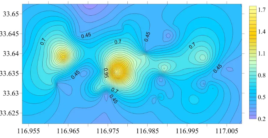
Moreover, in comparison with Fig. 2, the contour map of the cadmium concentrations of the environmental baseline samples shows only two areas with high cadmium concentrations (left and central), and the right one is disappeared (Fig. 4), this result indicates that the right area with high cadmium concentrations is a hotspot with high degree of anthropogenic contribution.

Fig. 4 Contour map of environmental baseline

CONCLUSION

Based on the spatial and statistical analyses of the cadmium concentrations in the shallow groundwater collected from the urban area of Suzhou, northern Anhui Province, China, the following conclusions have been made:

(1) The groundwater samples show good quality based on their cadmium concentrations, and three areas with high relative concentrations of cadmium have been identified, which might be indication of anthropogenic effects; (2) Spatial and statistical methods have identified fifteen outliers, which are considered to be samples with extreme high values or different with their neighborhoods;

Acknowledgement

This work was financially supported by National Natural Science Foundation of China (41302274 and 41173106), and the National College Students Innovation and Entrepreneurship Training Program of China (201210379026). Samples were collected by GX Chen, XX Chu and GF Lin from the Suzhou University.

REFERENCES

[1] LH Sun, HR Gui, DS Xu, SL Huang, Fresenius Environmental Bulletin, 2012, 21(2), 263-268.

[2] P Wongsasuluk, S Chotpantarat, W Siriwrong, M Robson, Environmental Geochemistry and Health, 2014, 36, 169-182.

[3] CEPA (Chinese Environmental Protection Administration), Elemental background values of soils in China, Beijing: Environmental Science Press, 1990.

[4] LH Sun, HR Gui, WH Peng, ML Lin M, Nature Environment and Pollution Technology, 2013, 12(3), 533-536. [5] A Molinari, L Guadagnini, M Marcaccio, A Guadagnini, Science of the Total Environment, 2012, 425, 9-19. [6] R Salminen, T Tarvainen, Journal of Geochemical Exploration, 1997, 60(1), 91-98.

[7] C Reimann, RG Garrett, Science of the Total Environment, 2005, 350(1), 12-27. [8] A Gałuszka, Environmental Geology, 2007, 52(5), 861-870.

[9] Z Nakic, K Posavec, A Bacani, Ground Water, 2007, 45(5), 642-647.

[10] B Urresti-Estala, F Carrasco-Cantos, I Vadillo-Pérez, P Jiménez-Gavilán, Journal of Environmental

Management, 2013, 117, 121-130.

[11] Z Wang, I Chai, Y Wang, Z Yang, H Wang, X Wu, Environmental Monitoring and Assessment, 2011, 175(1-4), 167-173.

[12] PK Pandey, Y Verma, S Choubey, M Pandey, K Chandrasekhar, Bioresource Technology, 2008, 99(10), 4420-4427.

[13] WHO (World Health Organization), Guidelines for drinking-water quality (3rd edition), Geneva: World Health Organization, 2008.

[14] RM Lark, Geoderma, 2002, 106, 173-190.