Multi-objective Evolutionary Algorithms and Hyper-heuristics for
Wind Farm Layout Optimisation
Wenwen Li, Ender ¨Ozcan, Robert John
Automated Scheduling, Optimisation and Planning (ASAP) Research Group
University of Nottingham, School of Computer Science, Jubliee Campus, Wallaton Road, Nottingham NG8 1BB, UK
Abstract
Wind farm layout optimisation is a challenging real-world problem which requires the discovery
of trade-off solutions considering a variety of conflicting criteria, such as minimisation of the land
area usage and maximisation of energy production. However, due to the complexity of handling
multiple objectives simultaneously, many approaches proposed in the literature often focus on the
optimisation of a single objective when deciding the locations for a set of wind turbines spread
across a given region. In this study, we tackle a multi-objective wind farm layout optimisation
problem. Different from the previously proposed approaches, we are applying a high-level search
method, known as selection hyper-heuristic to solve this problem. Selection hyper-heuristics mix
and control a predefined set of low-level (meta)heuristics which operate on solutions. We test nine
different selection hyper-heuristics including an online learning hyper-heuristic on a multi-objective
wind farm layout optimisation problem. Our hyper-heuristic approaches manage three well-known
multi-objective evolutionary algorithms as low-level metaheuristics. The empirical results indicate
the success and potential of selection hyper-heuristics for solving this computationally difficult
problem. We additionally explore other objectives in wind farm layout optimisation problems to
gain a better understanding of the conflicting nature of those objectives.
Keywords: Wind farm, Layout design, Optimisation, Hyper-heuristics, Evolutionary algorithms, Operation research
1. Introduction
Wind power is an increasing source of renewable energy, harnessed through wind turbines on
onshore and offshore areas. 320 Gigawatts (GW) of wind power capacity, doubling the figure in
2014, is expected to be installed in Europe by 2030 [1]. The wind farm layout optimisation (WFLO)
problem involves determining the best locations for wind turbines in a given region considering
certain objectives subject to a variety of constraints. WFLO is a computationally difficult problem
to solve, and a crucial goal is minimising the cost of energy (COE) which has been extensively
studied in the scientific literature [2]. COE embeds multiple components under a single objective
formulation, including installed capital cost, annual operation and maintenance cost, the number
of turbines, the annual energy production (AEP) and more. In some studies, researchers and
practitioners focus on improving AEP as a single objective due to its relatively considerable effect
on COE [3]. Hence, the positions of turbines are optimised to maximise AEP. Then again, AEP
gets influenced by several other key factors, such as wind source, terrain conditions, type, number
and spacing of wind turbines, etc.
In this paper, we deal with one of the multi-objective WFLO problem variants adopted from [4].
AEP is maximised through the minimisation of wake loss. Instead of using the classical approach
of applying a multi-objective evolutionary algorithm (MOEA) to solve the multi-objective WFLO
problem, we demonstrate the effectiveness and potential ofselection hyper-heuristics(Section 2.3) as solution methods, exploiting the strengths of multiple MOEAs. Moreover, we explore the conflicting
nature of several objectives including minimisation of COE, maximisation of AEP and minimisation
of the number of turbines under a multi-objective hyper-heuristic framework.
Our motivations for conducting this work are as follows. Firstly, MOEAs utilise different
strate-gies for balancing exploration (capability of jumping to a different region in the search landscape
where the global optimum is potentially located whenever needed) and exploitation (capability
of performing local search) while searching the solution space (Section 2.1). Thus, this provides
us with a research question - can we combine the strengths of different MOEAs to solve unseen
problem instances? Secondly, there is a growing number of studies reporting the effectiveness of
selection hyper-heuristics as general purpose solution methods for a range of computationally
dif-ficult real-world problems from educational timetabling to vehicle routing [5]. Thirdly, to the best
of the authors’ knowledge, there has been no studies on hyper-heuristics for solving multi-objective
This work is organised as follows. We first provide a background on general multi-objective
optimisation problems, related work on multi-objective WFLO problems and hyper-heuristics in
Section 2. Then we formulate our multi-objective WFLO problem model in Section 3. Our
method-ologies are presented in Section 4. The experimental design and empirical results are discussed in
Section 5. More insights of different trade-offs in multi-objective WFLO problems are explored in
Section 6. Finally, our conclusion and future work are in Section 7.
2. Background and Related Work
2.1. Multi-objective Optimisation Problem (MOP)
Definition 1. (MOP) Without loss of generality, we define an MOP as minimising a set (or a vector) of objectivesF(x), where F(x) = (f1(x), f2(x), . . . , fk(x). Suppose that a decision variable xi is a d-dimensional vector, say, xi = [x1i, x
2 i, . . . , x
d
i] and a solution x consists of a vector ofn
decision variables.
minimise [F(x) = (f1(x), f2(x), . . . , fk(x)]
subject to
gi(x)≤0 , i= 1,2. . . , m
hj(x) = 0, j= 1,2. . . , p
x= [x1, ..xi.., xn] x∈Ω
wheremis the number of inequality constraints andpis the number of equality constraints. Multiple
objectives can be combined under a single-objective formulation (e.g., via multiplication or weighted
average). The distinguishing difference between MOPs and single-objective optimisation problems
is that the approaches to former problems optimise a set of objectives simultaneously, eventually
providing a set of ‘trade-off’ solutions, namelyPareto Set, while the approaches to the latter only optimise one objective at a time providing a single resultant solution. The Pareto set contains
solutions whose one objective can not be improved without worsening at least one other objective.
The corresponding vectors of objectives form aPareto Front (PF) in the objective space.
Because of the real-world complexities of multi-objective problems, including large search space,
oper-ational research (OR) techniques often fail to produce “satisfactory” results. Hence, heuristic
optimisation methods, particularly multi-objective evolutionary algorithms (MOEAs) are widely
used for solving MOPs due to their ability in generating multiple solutions even in a single run and
being less sensitive to the varying geometries of PFs [6].
In this study, we have used three well-known MOEAs, Nondominated Sorting Genetic
Algorithm-II (NSGA-Algorithm-II) [7], Strength Pareto Evolutionary Algorithm 2 (SPEA2) [8] and Indicator-based
Evo-lutionary Algorithm (IBEA) [9]. Each approach employs a different strategy for preserving the
diversity of solutions during the search process and so perform ranking, selecting and replacing
(or truncating) solutions, differently. More specifically, NSGA-II uses a fast non-dominated sorting
to rank the solutions, and assigns a crowding distance (a measure of the density of solutions for any specific PF) to each solution. SPEA2 assigns a ‘fitness’ to each solution considering the
num-ber of individuals which dominates that solution and the distance to the k-th nearest neighbour.
Moreover, this approach iteratively removes a solution which has the minimum distance to its
k-th nearest neighbour until k-the size of k-the current population reduces to a predefined parameter
population size. IBEA ranks solutions based on their contributions to the performance indicator in use, such as hypervolume or indicator [9]. The solution with the least contribution in the
population is removed one at a time to maintain the fixed population size. Each algorithm shows a
different behaviour during the search process due to their differing components. Their behaviours
on a WFLO benchmark are presented in Section 5.2.
In a single-objective optimisation problem, the quality of solutions can be directly assessed by an
evaluation function. However, there is no clear criterion regarding how to evaluate a population of
trade-off solutions generated by different MOEAs. Therefore, many quality indicators are designed
to assess the PFs containing trade-off solutions from different perspectives.
In this study, the following indicators are used: size of space covered (SSC), also know as
S-matrix or hypervolume [10], uniform distribution (UD) [11], ratio of non-dominated Individual (RNI) [11] and algorithm effort (AE) [11]. Hypervolume is defined as the space covered by a PF
with respect to a reference point (also known as an inferior point). It is usually used to evaluate
a multi-objective algorithm’s convergence ability. UD, a value in [0,1], measures the uniformity
of the distribution of non-dominated individuals on the PF. A higher value of UD indicates that
the solutions on a PF are distributed more uniformly. RNI, a value in [0,1], is the percentage of
in second. Each indicator illustrates the strength of an MOEA from a different view. The higher
the value, the better the performance of an algorithm is with respect to the given indicator. A
comprehensive review of quality indicators used in MOEAs can be found in [12]. More on MOEAs
can be found in [6].
2.2. Related Work on Multi-objective WFLO Problems
Kusiaket al.[13] modelled a bi-objective WFLO problem, i.e. maximising the energy production and minimising the constraint violation of the minimum inter-distance between any two turbines,
and solved it by Strength Pareto Evolutionary Algorithm (SPEA) [10]. Veeramachaneniet al. [14] presented a Multi-objective Particle Swarm Optimisation (MOPSO) algorithm which combined
a general purpose MOPSO [15] algorithm with problem-specific repair strategies to maximise the
energy capture and minimise the layout cost. The layout cost was modelled in terms of the land area
usage and the number of turbines. Kwonget al. [16] considered minimising the noise production while maximising the energy production in their bi-objective model, using General NSGA-II to
solve this problem. Tong et al.[17] proposed a bi-level multi-objective WFLO framework which maximised the wind farm annual capacity factor and the land area per MW installed. The authors
reformulated this bi-objective problem as a constrained single-objective optimisation problem and
applied Mixed-Discrete Particle Swarm Optimization (MDPSO) to solve this reformulated problem.
A real case study was presented in Csicsbot et al. [18]. The authors utilised a multi-objective genetic algorithm (GA) to obtain an optimal placement of wind turbines by maximising the power
production while restricting the budget of installed turbines in the Gokceada Island onshore wind
farm. Tran et al.[4] designed problem-specific crossover and mutation operators and embedded them in three general MOEAs (NSGA-II, SPEA2 and IBEA) individually to solve a three-objective
WFLO problem with different numbers (30, 50, 70 and 200) of turbines. More details about their
problem model are in Section 3.
A comprehensive literature review of the WFLO problem and methodologies in use can be found
in [2].
2.3. Hyper-heuristics
A metaheuristic, such as a GA or particle swarm optimisation, is“a high-level problem-independent algorithmic framework that provides a set of guidelines or strategies to develop heuristic optimisa-tion algorithms” [19]. Based on this recent definition, hyper-heuristics can be considered as a subset of metaheuristics. The distinguishing feature of hyper-heuristics is that they, as high-level methods,
perform search over the space formed by a set of low-level heuristics which explore the space of
solutions. The low-level heuristics can be (neighbourhood) operators, such as crossover, mutation,
local search, or they could be themselves metaheuristics.
There is a logical separation between the high-level hyper-heuristic control strategy and low-level
(meta)heuristics under the originally proposed framework, enabling component based development
[20]. A hyper-heuristic is allowed to access problem domain independent information (such as the
objective value of a solution) and perform some bookkeeping (such as maintaining performance
indicator(s) for each low-level (meta)heuristic). The advantage of using hyper-heuristics is that
the same method or its components can be reused without requiring any change, assuming that
the low-level (meta)heuristics are already implemented. Even, the low-level (meta)heuristics are
replaceable.
Hyper-heuristics can be categorised in different ways with respect to different criteria.
Con-sidering the nature of the heuristic search space, two main types of hyper-heuristics have been
observed: (1)heuristic selectionmethods that choose one of the low-level (meta)heuristics to apply at a given time and (2) heuristic generation methods for generating new (meta)heuristics from given components. From the number of incumbent solutions used during the search process
per-spective, hyper-heuristics perform single-point based or multi-point based search. The majority of
hyper-heuristic studies are on selection hyper-heuristics which perform single-point based search
[5] improving a single complete solution, iteratively. In this framework, first, one of the low-level
(meta)heuristics is chosen based on a certain selection strategy. Then, this low-level (meta)heuristic
is applied to a single candidate solution to generate a new solution. After that, a decision is made
on whether to accept or reject this new solution based on a certain acceptance strategy. Thus, this
framework consists of two main components: (1) heuristic selection method and (2) move
accep-tance method as identified by Bilginet al.[21] and ¨Ozcanet al.[22]. Both components are executed iteratively until termination. Each iteration is referred to as a “decision point” (DP).
On the other hand, there are a few studies on selection hyper-heuristics which perform
multiple solutions for a number of steps. In this study, we focus on such selection hyper-heuristics
performing multi-point based search in the context of multi-objective optimisation. The choice
function based multi-objective hyper-heuristic proposed by Maashiet al. [23] is one of the limited studies in this area. An on-line learning mechanism based on four quality indicators (see Section
4.2.3) is designed to select an appropriate MOEA to perform at each DP. Two different move
acceptance strategies: Great Deluge Acceptance [24] and Late Acceptance (LA) [25, 26] are modified
to solve MOPs [27].
The empirical results demonstrate the effectiveness and advantages of solving continuous MOPs
compared to underlying MOEAs (NSGA-II, SPEA2 and MOGA [28]) both on Walking Fish Group
(WFG) benchmark problems and a real-world problem - vehicle crashworthiness problem. A brief
review of other multi-objective hyper-heuristic approaches is presented in [23]. A recent review of
hyper-heuristics both on single-objective and multi-objective can be found in [5].
3. Problem Formulation
The three-objective WFLO problem presented by Tran et al. [4], is tackled in this study to obtain the best locations for a given number of turbines on the WF area. The three objectives are
to maximise the energy production and minimise both the cable length connecting all turbines and
the land covered by the turbines within the given WF area. Two constraints are considered, i.e.
wind farm boundary constraint (no turbine can be placed outside the given WF area) and minimum
turbine spacing constraint (any two turbines cannot be placed within a certain distance, that is,
eight times the rotor radius in this case). The decision variables are the positions of n turbines in a
given WF denoted as an array of 2D coordinates (X,Y) = [(x1,y1),(x2,y2), . . . ,(xi,yj), . . . ,(xn,yn)],
where (xi,yi) is the position of the ith turbine.
The problem formulation is as follows. Given a rectangular wind farm with length l, width w
minimise{1/E(P), M ST, A}
subject to
1≤xi ≤l,1≤yi ≤w , i∈[1, . . . , n]
q
where MST is the cable length computed using the Prim’s Minimum Spanning Tree algorithm
[29], considering that each turbine is a node, and the Euclidean distance between each pair of
turbines represents the weight on each arc of an undirected weighted graph. A is the used land
area determined by the convex hull of turbine locations which are computed using the Grahams
algorithm [30], E(P) is the total expected energy production from this WF using a given layout, R
is the rotor radius of a wind turbine.
E(P) is given by Eq. (1).
E(P) =X
i Z
θ
P(θ) Z
v
f(v)p(v(θ), κ, ci(θ, X, Y))), (1)
where v is the wind speed following a Weibull distribution represented by p(v(θ), κ,ci(θ,X,Y))
estimated from the wind data considering turbine locations (X,Y), and P(θ) represents the
proba-bility distribution of the wind source as a function of wind directionθ. The energy production of
each turbine contributing to E(P) varies depending on the wake effect caused by nearby turbines.
Park model [13] is utilised to calculate this wake effect. In this model, the wake effect reduces the
wind sources available on a turbine i by decreasing the scale parameter c of the estimated Weibull
distributed wind source for the whole WF (also known as free-stream wind source). Hence, each
turbine has its scale parameter ci. The shape parameter κis not affected for any turbine in this
model. The scale parameterci(θ) is decided by the velocity deficit that turbine i experienced from
the nearby turbines in the wind direction θ. The reduced wind speed on each turbine i in each
wind directionθinfluences the power output of that turbine. A sigmoid power curve function f(v)
is used in this model. More specifically, if the wind speed is smaller than the cut-in speed or greater
than the cut-out speed, no energy is produced. If the wind speed is between the cut-in speed and
the rated speed, the power output follows a linear function. If it is within the range of the rated
speed and the cut-out speed, then the turbine generates its rated power. The readers can find more
details on the calculation of E(P) in [13].
4. Methodologies
In this section, we present the details of the framework enabling the use of multi-objective
4.1. MO HH Framework
The general algorithmic framework for the MO HHs used in the experiment is provided in
Algorithm 1. First, initialisation process, including generation of initial solutions and setting up
of the relevant data structures of the selection hyper-heuristic takes place (Step 2). This process
is followed by iterative improvement of a population of trade-off solutions using multiple
multi-objective metaheuristics. At each DP, an MOEA is chosen using the metaheuristic selection method
(Step 4) and applied (Step 5) to the input set of solutions (Pin) for a fixed number of steps (i.e.,
generations), producing a set of new solutions (Pnew). Then some data/parameters relevant to
algorithmic components get updated (Step 6), which is followed by move acceptance (Step 7),
deciding the next input population from the pool of solutions formed by the union of current and
newly generated solutions for the next DP. This whole process terminates after iterating for a fixed
number of DPs, and the Pareto set is returned.
The initialisation (Step 2) and update (Step 6) processes are used by choice function MO HHs
to initialise and update the utility (choice function) score of each MOEA when a new population
is generated, respectively. More explanations can be seen in Section 4.2.3. No initialisation and
updating schemes are required by the fixed sequence or random choice MO HHs.
Algorithm 1:MO HH Framework
1 h: index of the chosen heuristic;Pin: input population;Pnew: newly generated population;
2 Initialise();
3 while(!stop criteria are satisfied) do
4 h←ChooseMOEA() ;
5 Pnew←ExecuteMOEA(h,Pin,g);
// execute MOEA h for g generations using input population Pin to produce
a new population Pnew
6 Update();
7 Pin←ApplyMoveAcceptance(Pnew,Pin);
// use AM, GDA or BA as the move acceptance strategy
4.2. Heuristic Selection Methods
In this study, well known and modified heuristic selection methods as selection hyper-heuristic
components are used for choosing the right multi-objective metaheuristic at each DP.
4.2.1. Random Choice (RC)
This method simply chooses a random low-level metaheuristic. It is usually used as a
refer-ence approach for performance assessment of the learning hyper-heuristic methods. The initial
population of solutions are created randomly.
4.2.2. Fixed Sequence (FS)
Considering that the low level (meta)heuristics are chosen and applied one after and other
dur-ing the search process, it has been of interest to find a good sequence (or sequences) of low-level
(meta)heuristics for a given problem instance [5]. A simple approach would be making use of
low-level (meta)heuristics in a predefined sequence. This (meta)heuristic selection method utilises a
fixed permutation of low-level (meta)heuristics, where each (meta)heuristic is executed
consecu-tively in that order. The initial set of solutions is randomly produced.
4.2.3. Choice Function (CF)
The CF heuristic selection method proposed by Maashiet al. [23] assigns a score to each low-level metaheuristic indicating its performance and the metaheuristic with the maximum score is chosen
at each DP. This approach intends to balance intensification (choosing the best performing low-level
metaheuristic) and diversification (giving a chance to a metaheuristic which is not selected for a long
time) in one function. The CPU seconds elapsed since the last call to a low-level (meta)heuristic
serve as the diversification component, while the intensification part is modelled using a two-stage
ranking scheme.
In the first stage of the scheme, each MOEAs is ranked with multiple quality indicators
sepa-rately, in particular, hypervolume, RNI, UD, and AE. The second stage uses the frequency of best
quality indicators that each MOEA achieves. Suppose that the framework contains three different
MOEAs denoted as h1,h2,h3, if h1 achieves the best rank in hypervolume, UD and RNI, h2 also
performs best in RNI and UD, while h3 only gets the best rank in hypervolume, the frequency
The final score (or value) for a given MOEA (h) is computed by the CF function Eq. (2).
CF(h) =αf1(h) +f2(h),∀h∈H (2)
where α is a positive valued parameter, H contains all indices of MOEAs, h is the index of an
MOEA. The intensification component (f1) is defined as
f1(h) = 2(N+ 1)− {F reqrank(h) +RN Irank(h)} (3)
where N is the total number of MOEAs. Freqrank(h) is the rank of the frequency count of the
best-ranked indicators of heuristic h, RNIrank(h) is the RNI rank of h. Following the above example, we
know RNIrank(h) = 1,1,3; combining the Freqrank(h) = 1,2,3 for each MOEA, we can get f1(h) =
6,5,2 for h1,h2,h3respectively. f2(h) is the elapsed CPU time (in seconds) since the time h was last
called. MOEA with the highest value from CF is selected.
The initialisation scheme for the Choice Function based MO HHs is a greedy strategy which
executes each MOEA h for a fixed number of generations and then computes all four indicators
(hypervolume, RNI, UD and AE) individually to initialise the two-stage ranking mechanism as
explained above. MOEA with the highest CF value (calculated by Eq. (2) is chosen as the initial
h to be applied starting the search process.
4.3. Move Acceptance Methods
Move acceptance methods play an important role in hyper-heuristics by deciding whether to
accept or reject candidate solution(s) produced by the selected heuristic. There are many various
simple and elaborate move acceptance methods used as a part of metaheuristics in single objective
optimisation. Maashiet al. [27] modified and evaluated two such elaborate move acceptance for multi-objective optimisation: GDA and LA. However, since the empirical results showed that LA
does not perform well, it is not used in this study.
4.3.1. All-Moves (AM)
All solutions generated by the selected metaheuristic are accepted.
4.3.2. Great Deluge Acceptance with D metric (GDA)
Great Deluge Algorithm was originally designed by Dueck [31] for single objective problems.
which is referred as Water Level. The threshold increases linearly with a fixed step parametrised as UP every time after a solution is accepted. This algorithm is integrated into hyper-heuristics as
an acceptance strategy in various single objective hyper-heuristic approaches. Maashi et al. [27] modified this acceptance strategy to adapt to multi-objective hyper-heuristics by usingD metric
[32] as the indicator to decide whether to accept or reject the candidate population. The D metric
measures the objective space coverage difference between two fronts. For example, D(A, B) is the
space covered by front A, but not by B. The pseudo code of GDA is shown in Algorithm 2.
Algorithm 2:GDA Pseudo Code
1 A: the previous accepted front;B: the newly generated front;LEV EL: water level,
initialised with a small value;
2 D(B, A) =SSC(A+B)−SSC(A);
// space only covered by B, not by A
3 if (D(B,A)>LEVEL) then 4 A:=B;
5 LEV EL=LEV EL+U P;
4.3.3. Best Acceptance
A simple way of using the idea of only-improving move acceptance strategy in a multi-objective
optimisation framework would be to accept the ‘best’ set of solutions maintaining history. In this
study, we present the Best Acceptance (BA) which ranks all the solutions from the pool of the newly
generated solutions and the population of recently accepted. Then the ‘best’ n solutions (where n
is the population size) are allowed to survive as the input population for the next DP, requiring the
use of ranking and other supporting functionalities. Any of the three underlying MOEAs’ ranking
and truncating mechanisms (removal of excess solutions whenever the size of the population exceeds
n) can be applied in this best acceptance strategy. In this work, we use the NSGA-II’s ranking and
truncating mechanism.
Due to the stochastic nature of operators (e.g., crossover, mutation), they may generate solutions
which have already existed in previous populations. These duplicate solutions can degrade the
pseudo code of BA is shown in Algorithm 3.
Algorithm 3:BA Pseudo Code
1 AandB are two Pareto fronts.;
2 U nion:= Merge(A,B);
3 U nionnew ←Remove duplicated solutions inU nion;
4 while(U nionnew.size()>Population Size)do
5 Rank the solutions using the NSGA-II ranking mechanism ;
6 Remove the worst solution inU nionnewbased on crowding distances;
7 return: U nionnew;
5. Experiments
In this study, our goal is to evaluate and compare the performances of different multi-objective
hyper-heuristic approaches mixing/controlling three MOEAs {NSGA-II, SPEA2, IBEA} as
low-level metaheuristics.
5.1. Experimental Design
Wind turbine parameters are fixed as provided in [13]. The rotor radius is set to 38.5 m, cut-in
speed to 3.5 m/s, rated speed to 14 m/s, rated power to 1.5 MW and height to 80 m. A real world
wind scenario (scenario 2) from [13] is used in this work. The wind farm is restricted to a land area
of 3×3 km2and 30 turbines are to be placed within this area.
The algorithmic parameters of the MOEAs used in this work are set to the same values as
provided in [4], i.e. population size to 50, archive size to 50, total solution evaluations to 20000.
Problem specific operators (block swap crossover and movement mutation) designed by Tranet al.
[4] are utilised in all the algorithms in this work, with the crossover probability of 0.3 and mutation
probability of 0.9.
Our hyper-heuristics approaches are conducted using five different DP settings in{10, 20, 30, 40,
50}. For Choice Function based MO HHs, 1000 solutions for each MOEA are used to initialise the
two-stage ranking scheme in order to select the initial heuristic to be applied. No such initialisation
The parameterαfor Choice Function based MO HHs and UP for the GDA strategy are tuned
referring to the ranges of both parameters provided in [33] in different DP settings. More specifically,
αis set as 10 for the Choice Function based MO HHs. UP is set as 0.01 for 10 DPs, 0.003 for 20
and 30 DPs, 0.0003 for 40 and 50 DPs. Distance sharingσshare in UD quality indicator is set as
0.01 in normalized space as in [23]. The reference point for hypervolume (S metric) and D metric
regarding 30 turbines’ experiments is (area: 9 km2, energy production: 10526 KW, cable length: 17
km). This reference point is set based on trial runs of single MOEAs choosing the highest (worst)
value of each objective.
Each algorithm is executed for 30 independent trials on a computer with 64-bit Intel Core i3
3.4GHz\8G\120G configuration. Non-parametric statistical test - one-sided Wilcoxon Rank-Sum
Test (also known as MannWhitneyWilcoxon U test) is applied to determine whether there is any
statistically significant performance difference between two algorithms with respect to hypervolume.
The confidence level is set as 95%.
5.2. Results and Observations
In this section, we compare the performances of selection hyper-heuristics as well as the three
individually executed MOEAs with respect to different quality indicators, including{Hypervolume,
RNI, UD}. As we mentioned in Section 4.3.3 that except the MO HHs embedding BA, all
hyper-heuristics could have duplicate solutions in a population which are undesirable. More duplicate
solutions suggest a decrease in the strength of the corresponding algorithm in preserving
poten-tially more useful solutions. Thus, additional to those three quality indicators mentioned earlier,
we propose and use another performance metric, i.e. ratio of duplicated non-dominated individu-als (RDI), denoting the percentage of duplicate non-dominated solutions in the final population produced by an algorithm.
Table 1 summarises the experimental results comparing the performance of MO HHs and
MOEAs for the WFLO problem instance based on those four metrics. The best performance with
respect to the hypervolume is achieved by the random choice - great deluge acceptance (RC-GDA)
hyper-heuristic. For the Fixed Sequence MO HHs, the permutation of<SPEA2, NSGA-II, IBEA>
performs ‘slightly’ better than the rest of the permutations obtaining the highest hypervolume (Due
to the space limitation, we skip the empirical results from those experiments.). The experimental
Table 1: Performance of individual MOEAs and hyper-heuristics with 10 DP setting for 30 turbines based on different
metrics. The higher hypervolume, RNI and UD, the better. The smaller RDI, the better. ‘-’ means 0.ST Dindicates
standard deviation.
Hypervolume RNI RDI UD
MeanST D Median MeanST D Median MeanST D Median MeanST D Median
CF-AM 11.07430.1505 11.1137 0.93550.0538 0.9394 0.30730.0902 0.3163 0.46490.1189 0.4363
CF-GDA 11.12280.0700 11.1271 0.92650.0511 0.9384 0.30130.0677 0.2970 0.48870.0611 0.4913
CF-BA 11.14890.0862 11.1519 0.99930.0036 1.0000 - - 0.83280.0981 0.7849
FS-AM 11.21140.0692 11.2045 1.00000.0000 1.0000 - - 0.99450.0297 1.0000
FS-GDA 11.21780.0911 11.2286 0.99270.0254 1.0000 0.02840.0861 - 0.94700.1450 1.0000
FS-BA 11.20820.0661 11.2001 1.00000.0000 1.0000 - - 0.88430.0905 0.8348
RC-AM 11.10070.1504 11.1340 0.97900.0392 1.0000 0.12740.1577 0.0600 0.74000.2393 0.7122
RC-GDA 11.22840.1127 11.2322 0.97700.0354 1.0000 0.17960.1811 0.1000 0.71040.2661 0.6838 RC-BA 11.20120.1416 11.1986 1.00000.0000 1.0000 - - 0.87660.0968 0.8348
NSGA-II 10.58380.0946 10.5783 1.00000.0000 1.0000 0.08600.0302 0.0800 0.69530.0220 0.6986
SPEA2 10.88300.0813 10.8723 1.00000.0000 1.0000 - - 1.00000.0000 1.0000
IBEA 11.02930.3511 11.1258 0.94530.0430 0.9623 0.41500.0543 0.4200 0.44140.0585 0.4329
The statistical test between any pair of algorithms with respect to hypervolume is shown in
Tab. 2.
Behaviour of MOEAs: IBEA performs significantly better than NSGA-II and SPEA2 considering hypervolume. However, due to the lack of diversity mechanism in IBEA, the median RDI of the final
population is 42%. This value is much higher than those of the NSGA-II and SPEA2 approaches,
which are 8% and 0%, respectively. Considering that IBEA has the highest RDI, it is reasonable
that it has the lowest UD.
SPEA2 has a similar ability of generating non-dominated solutions (RNI) in a population as
NSGA-II, but SPEA2 converges better (a higher hypervolume) and the solutions spread more
uniformly (a higher UD) than NSGA-II. IBEA converges the best (the highest hypervolume) among
all the three MOEAs, but with limited ability of generating diversified solutions (a lower RNI and
UD) than SPEA2 and NSGA-II.
Table 2: Wilcoxon Rank Sum Test of hypervolume between any two algorithms. ‘<’ means significantly worse than;
‘≤’ indicates slightly worse than; ‘>’ means significantly better than; ‘≥’ is slightly better than. The comparison
direction is rows versus columns. For example, CF-GDA is slightly better (‘≥’) than CF-AM.
CF-AM CF-GDA CF-BA FS-AM FS-GDA FS-BA RC-AM RC-GDA RC-BA NSGA-II SPEA2
CF-AM
CF-GDA ≥
CF-BA > ≥
FS-AM > > >
FS-GDA > > > ≥
FS-BA > > > ≤ ≤
RC-AM ≥ ≥ ≤ < < <
RC-GDA > > > ≥ ≥ ≥ >
RC-BA > > ≥ ≤ ≤ ≤ > ≤
NSGA-II < < < < < < < < <
SPEA2 < < < < < < < < < >
IBEA ≥ ≤ ≤ < < < ≤ < < > >
better performance when compared to NSGA-II and SPEA2 with respect to hypervolume. The
same phenomena have been observed for IBEA for most of the cases. However, the performances of
CF based MO HHs and RC combined with all-move acceptance strategy (RC-AM hyper-heuristic)
are ‘slightly’ better than IBEA with respect to hypervolume (with no statistical significance).
Random Choice and Fixed Sequence MO HHs also achieves higher RNI and UD than the single
MOEA which suggests that both selection MO HHs exhibit a better diversification ability. From
the move acceptance perspective, BA and GDA perform similarly considering hypervolume, but
both of them are significantly better than AM when combined with CF and RC metaheuristic
selection methods.
To develop a further understanding regarding why selection hyper-heuristics, particularly,
Ran-dom Choice and Fixed Sequence MO HHs outperform each of the three MOEAs with respect to
hypervolume, we have arbitrarily chosen RC-GDA to visualise the PFs generated by this approach
as opposed to the ones obtained by each MOEA. The non-dominated solutions obtained by
RC-GDA, NSGA-II, SPEA2 and IBEA over 30 trials are collected, and then projections of Pareto fronts
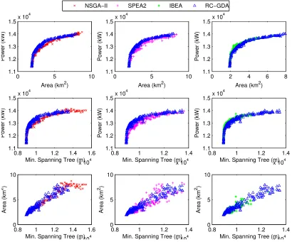
are plotted using the following combinations of objectives:
• maximisation of the power output and minimisation of the minimum spanning tree
• minimisation of the land area usage and minimum spanning tree
Figure 1 shows the comparison between RC-GDA and underlying MOEAs. Note those points
that ‘look like’ dominated by others on the same front (i.e. with the same colour) are not dominated
since they have better performance on the third objective.
0 2 4 6 8
1.1 1.2 1.3 1.4 1.5x 10
4
Area (km2)
Power (kW)
0.8 1 1.2 1.4
x 104 1.1
1.2 1.3 1.4 1.5x 10
4
Min. Spanning Tree (m)
Power (kW)
0.8 1 1.2 1.4
x 104 0
5 10
Min. Spanning Tree (m)
Area (km
2 )
0 5 10
1.1 1.2 1.3 1.4 1.5x 10
4
Area (km2)
Power (kW)
0.8 1 1.2 1.4 1.6 x 10⁴ 1.1
1.2 1.3 1.4 1.5x 10
4
Min. Spanning Tree (m)
Power (kW)
0.8 1 1.2 1.4 1.6
x 104 0
5 10
Min. Spanning Tree (m)
Area (km
2 )
0 5 10
1.1 1.2 1.3 1.4 1.5x 10
4
Area (km2)
Power (kW)
0.8 1 1.2 1.4
x 104 1.1
1.2 1.3 1.4 1.5x 10
4
Min. Spanning Tree (m)
Power (kW)
0.8 1 1.2 1.4
x 104 0
5 10
Min. Spanning Tree (m)
Area (km
2 )
[image:17.612.90.500.206.547.2]NSGA−II SPEA2 IBEA RC−GDA
Figure 1: Pareto front projections obtained from NSGA-II, SPEA2, IBEA and RC-GDA considering three different
combinations of objectives: Power-Area, Power-Minimum Spanning Tree and Area-Minimum Spanning Tree.
We can see that the PF of RC-GDA clearly dominates PFs generated by NSGA-II and SPEA2
both from convergence and spread perspectives. However, RC-GDA does not converge better than
better than the IBEA considering hypervolume.
RC-GDA mixes all three MOEAs which gives better chance to explore different regions of a
PF produced at each DP, resulting in more diversified solutions and better hypervolume than only
using a single MOEA, possibly because different MOEAs have strengths of exploiting and exploring
different regions of a PF. In our case, IBEA tends to exploit the region of the PF which maximises
AEP within a small land area (i.e. 2 to 5 km2), while NSGA-II and SPEA2 have better performance
of exploring the regions which maximise AEP in a larger land area (i.e. 2 to 9 km2). In other words,
different MOEAs can work together achieving a better trade-off solutions, eventually.
Apart from that, a strong positive linear correlation between the two objectives, i.e. minimising
the minimum spanning tree and the land usage is observed in Fig. 1. More specifically, the Pearson
product-moment correlation coefficients (PPMCC) [34] of both objectives for the resultant
trade-off solutions obtained from NSGA-II, SPEA2, IBEA and RC-GDA are 0.9628, 0.8771, 0.9021 and
0.9661 respectively, where this value is in [-1,1], and 1 represents total positive correlation. The
high PPMCCs suggest that it is potentially redundant to optimise both of those objectives under
a multi-objective problem formulation and perhaps one of the objectives can be ignored or both
can be merged into a single objective. It is evident that multi-objective WLFO models should be
designed carefully.
6. Problem Exploration
Multi-objective WFLO problems can be modelled in various ways as briefly reviewed in Section
2.2. Our model, as formulated in Section 3, is to maximise AEP, minimise the cable length and the
land area by optimising the positions of a fixed number of turbines (30 turbines). Even though we
are not considering minimising COE or the number of turbines in our model, it is still of interest
to see how our solutions would be reflected on those two important objectives and the potential
trade-offs among these objectives.
To do this, we run one of our hyper-heuristics - Fixed Sequence (<SPEA2, NSGA-II, IBEA>)
-Best Acceptance using a serial of turbine numbers (20, 25, 30,. . ., 100) 30 trials each, utilising the
same parameters described in Section 5.1. Then we collect all the non-dominated solutions’ energy
production to compute the COE values for each turbine number setting.
Many variants of COE can be found in the scientific literature. In our analysis, we are using
Com-petition [35]. In the original comCom-petition model setting, every 30 turbines require one substation.
Since it is questionable to assume that every 30 turbines require one substation, we only keep this
setting in our first COE model, but not in the second one. The purpose of using these two variants
of COE models is to further investigate the effect of different COE models or settings on forming
PFs.
The first COE model with substation setting is formulated as Eq. (4).
COE1=
(Ct∗n+Cs∗f loor(mn))∗ES+COM∗n (1−(1 +r)−y)/r ∗
1
8760∗P (4)
where Economies of scale (ES) is defined as
ES= 2
3+ 1 3 ∗e
−0.00174n2
(5)
Ct=£487,500 per turbine cost1, n is the number of turbines. Cs=£5,200,000 is the cost per substation. m = 30 denotes that one substation is needed for 30 turbines. COM=£13,000 is the annual operation and maintenance cost per turbine. P is the energy output. 8760 is the total hours
in a year. r = 0.03 interest rate. y = 20 denotes a wind farm lifespan of 20 years.
The difference between COE1 (Eq. (4)) and GECCO’s original model is that GECCO’s model
has one more component – farm size coefficient 0n.1 in its formula which is mainly used to prevent
the situation of a search algorithm resulting with a solution producing an overall COE of 0 (at
minimum) by providing the option of no turbine use.
In our second COE model, we exclude the cost of substation as in Eq. (6).
COE2=
Ct∗n∗ES+COM∗n
(1−(1 +r)−y)/r ∗ 1
8760∗P (6)
where ES is the same as Eq. (5)
Several main findings from Fig. 2 are as follows. Firstly, clear ‘jumps’ in the COE values
considering substation are observed in Fig. 2(a). For every 30 turbine interval, the COE value is
the highest (worst) at the beginning of this interval since a new substation is added, then it decreases
because more power can be generated from more turbines. Secondly, Fig. 2(b) shows that the COE
1The original cost is in USD dollars, we convert all the prices from USD dollars to British Pounds using the ratio
0.5 1 1.5 2 2.5 3 3.5 4 4.5 x 10⁴ 6 6.5 7 7.5 8 8.5 9 9.5 10 10.5x 10
−3
Power (KW)
Cost of Energy (£/KWh)
20T 25T 30T 35T 40T 45T 50T 55T 60T 65T 70T 75T 80T 85T 90T 95T 100T
(a)COE1 against Power-with substation setting
0.5 1 1.5 2 2.5 3 3.5 4 4.5
x 104 5.5 6 6.5 7 7.5 8 8.5
9x 10 −3
Power (KW)
Cost of Energy (£/KWh)
20T 25T 30T 35T 40T 45T 50T 55T 60T 65T 70T 75T 80T 85T 90T 95T 100T
(b)COE2 against Power-without substation setting
Figure 2: (a) is the scatter of COE1 (with substation setting) against power output obtained from optimising the
positions of a serial number of turbine numbers. From left to right (colour from blue to red) is from 20T (turbines)
to 100T (turbines) and (b) is the scatter of COE2 (without substation setting) against power output.
values change with the increase of the energy production if no substation is considered in the COE
model. In the beginning, the COE values are slowly reduced, since more energy is produced as the
number of turbines increases. Then COE rises due to the more severe wake loss caused by more
installed turbines. This finding is also consistent with the observation in a wind energy industry
report [36].
Thirdly, both Fig. 2(a) and Fig. 2(b) suggest that there are indeed trade-offs among the
[image:20.612.213.405.106.346.2]of turbines. For example, in Fig. 2(a), although 25 turbines’ configuration gives the lowest COE
(COE1), the energy production is also relatively low which does not satisfy the goal of maximising
AEP or minimising the number of turbines (which can be 20 turbines or less). The horizontal
dash line in Fig. 2(b) illustrates a simple example of the trade-offs that for a given COE (COE2)
value, 35 turbines would be a more favourable choice if the decision maker(s) prefer to minimise the
number of turbines. Otherwise, 55 turbines (which has the same level of COE) would be a better
choice than say 35 turbines for the sole purpose of maximising the energy production.
Our analyses show two key findings. Firstly, COE, AEP and the number of turbines can be
formulated into a single-objective formulation. However, the use of multi-objective optimisation
ap-proaches would be more suitable, since we can still observe the multi-objective or conflicting nature
among these three objectives. Secondly, settings or modellings of COE influence the geometries of
PFs, and thus pose various difficulties for different MOEAs considering that each algorithm makes
use of different search components. For example, MOEAs without adequate diversification
mech-anisms can easily get trapped in a local optimum while searching a disconnected and multi-modal
PF, such as illustrated in Fig. 2(a).
7. Conclusion and Future Work
This study investigated the application of three state-of-the-art multi-objective evolutionary
algorithms, namely NSGA-II, SPEA2 and IBEA for solving a multi-objective wind farm layout
optimisation problem. The objectives include maximisation of the annual energy production,
min-imisation of the cable length and minimising the land area. We then tried to solve this
com-putationally difficult problem more effectively by mixing these three multi-objective evolutionary
algorithms using nine different selection hyper-heuristics. The empirical results indicated that
selec-tion hyper-heuristics could indeed exploit the strengths of multiple multi-objective metaheuristics,
and thus achieve statistically significant better performance than each constituent multi-objective
metaheuristic used on its own with respect to different performance indicators, including
hyper-volume and uniform distribution. This phenomenon has been verified by further analysing the
convergence and diversification properties of selection hyper-heuristics and the three underlying
metaheuristics based on their resultant Pareto fronts.
This work also studied the conflicting nature of three other objectives: minimising cost of energy,
behind this exploration is that the complexity of the wind farm layout optimisation problem calls for
the balance of various conflicting objectives, even though these objectives are sometimes formulated
into a single objective, such as cost of energy. Our analysis reveals that although annual energy
production and the number of turbines are often modelled as components into the formulation of
cost of energy, there are trade-offs among these three objectives and the modelling or setting of cost
of energy can affect the geometries of final Pareto fronts. Further investigations and insights into
the cost of energy models and the trade-offs among these three objectives would benefit decision
makers for wind farm development.
In the future, we plan to design and test more intelligent selection mechanisms and adaptive
move acceptance methods as components of multi-objective selection hyper-heuristics for solving
new multi-objective wind farm layout optimisation problem instances. The new problem instances
will be considered under different conflicting objectives subject to additional constraints, including
geographical constraints with more realistic shapes of wind farms.
References
[1] E. W. E. Association, Wind energy scenarios for 2030 (2015).
URL http://www.ewea.org/fileadmin/files/library/publications/reports/
EWEA-Wind-energy-scenarios-2030.pdf
[2] J. F. Herbert-Acero, O. Probst, P.-E. R´ethor´e, G. C. Larsen, K. K. Castillo-Villar, A review
of methodological approaches for the design and optimization of wind farms, Energies 7 (11)
(2014) 6930–7016.
[3] T. S, L. E, H. M, M. B, S. A, S. P, 2011 cost of wind energy review (2013).
URLhttp://www.nrel.gov/docs/fy13osti/56266.pdf
[4] R. Tran, J. Wu, C. Denison, T. Ackling, M. Wagner, F. Neumann, Fast and effective
multi-objective optimisation of wind turbine placement, in: Proceedings of the 15th annual conference
on Genetic and evolutionary computation, ACM, 2013, pp. 1381–1388.
[5] E. K. Burke, M. Gendreau, M. Hyde, G. Kendall, G. Ochoa, E. ¨Ozcan, R. Qu, Hyper-heuristics:
A survey of the state of the art, Journal of the Operational Research Society 64 (12) (2013)
[6] C. A. C. Coello, D. A. Van Veldhuizen, G. B. Lamont, Evolutionary algorithms for solving
multi-objective problems, Vol. 242, Springer, 2002.
[7] K. Deb, A. Pratap, S. Agarwal, T. Meyarivan, A fast and elitist multiobjective genetic
algo-rithm: Nsga-ii, IEEE transactions on evolutionary computation 6 (2) (2002) 182–197.
[8] E. Zitzler, M. Laumanns, L. Thiele, et al., Spea2: Improving the strength pareto evolutionary
algorithm, in: Eurogen, Vol. 3242, 2001, pp. 95–100.
[9] E. Zitzler, S. K¨unzli, Indicator-based selection in multiobjective search, in: Parallel Problem
Solving from Nature-PPSN VIII, Springer, 2004, pp. 832–842.
[10] E. Zitzler, L. Thiele, Multiobjective evolutionary algorithms: a comparative case study and
the strength pareto approach, evolutionary computation, IEEE transactions on 3 (4) (1999)
257–271.
[11] K. C. Tan, T. H. Lee, E. F. Khor, Evolutionary algorithms for multi-objective optimization:
performance assessments and comparisons, Artificial intelligence review 17 (4) (2002) 251–290.
[12] E. Zitzler, L. Thiele, M. Laumanns, C. M. Fonseca, V. G. Da Fonseca, Performance
assess-ment of multiobjective optimizers: an analysis and review, Evolutionary Computation, IEEE
Transactions on 7 (2) (2003) 117–132.
[13] A. Kusiak, Z. Song, Design of wind farm layout for maximum wind energy capture, Renewable
Energy 35 (3) (2010) 685–694.
[14] K. Veeramachaneni, M. Wagner, U.-M. O’Reilly, F. Neumann, Optimizing energy output and
layout costs for large wind farms using particle swarm optimization, in: Evolutionary
Compu-tation (CEC), 2012 IEEE Congress on, IEEE, 2012, pp. 1–7.
[15] X. Li, A non-dominated sorting particle swarm optimizer for multiobjective optimization, in:
Genetic and Evolutionary ComputationGECCO 2003, Springer, 2003, pp. 37–48.
[16] W. Y. Kwong, P. Y. Zhang, D. Romero, J. Moran, M. Morgenroth, C. Amon, Multi-objective
wind farm layout optimization considering energy generation and noise propagation with
[17] W. Tong, S. Chowdhury, A. Mehmani, A. Messac, Multi-objective wind farm design: Exploring
the trade-off between capacity factor and land use, in: Proceedings of the 10th World Congress
on Structural and Multidisciplinary Optimization, Orlando, FL, USA, 2013, pp. 19–24.
[18] S. S¸i¸sbot, ¨O. Turgut, M. Tun¸c, ¨U. C¸ amdalı, Optimal positioning of wind turbines on g¨ok¸ceada
using multi-objective genetic algorithm, Wind Energy 13 (4) (2010) 297–306.
[19] K. S¨orensen, F. W. Glover, Metaheuristics, in: S. I. Gass, M. C. Fu (Eds.), Encyclopedia of
Operations Research and Management Science, Springer US, 2013, pp. 960–970.
[20] P. Cowling, G. Kendall, E. Soubeiga, A hyperheuristic approach to scheduling a sales summit,
in: Practice and Theory of Automated Timetabling III, Springer, 2001, pp. 176–190.
[21] B. Bilgin, E. ¨Ozcan, E. E. Korkmaz, An experimental study on hyper-heuristics and exam
timetabling, in: Practice and Theory of Automated Timetabling VI, Springer, 2007, pp. 394–
412.
[22] E. Ozcan, B. Bilgin, E. E. Korkmaz, A comprehensive analysis of hyper-heuristics, Intelligent
Data Analysis 12 (1) (2008) 3.
[23] M. Maashi, E. ¨Ozcan, G. Kendall, A multi-objective hyper-heuristic based on choice function,
Expert Systems with Applications 41 (9) (2014) 4475–4493.
[24] G. Kendall, M. Mohamad, Channel assignment in cellular communication using a great
del-uge hyper-heuristic, in: Networks, 2004.(ICON 2004). Proceedings. 12th IEEE International
Conference on, Vol. 2, IEEE, 2004, pp. 769–773.
[25] E. K. Burke, Y. Bykov, A late acceptance strategy in hill-climbing for exam timetabling
prob-lems, in: PATAT 2008 Conference, Montreal, Canada, 2008.
[26] E. Ozcan, Y. Bykov, M. Birben, E. K. Burke, Examination timetabling using late acceptance
hyper-heuristics, in: Evolutionary Computation, 2009. CEC’09. IEEE Congress on, IEEE,
2009, pp. 997–1004.
[27] M. Maashi, G. Kendall, E. ¨Ozcan, Choice function based hyper-heuristics for multi-objective
[28] C. M. Fonseca, P. J. Fleming, Multiobjective optimization and multiple constraint handling
with evolutionary algorithms. i. a unified formulation, Systems, Man and Cybernetics, Part A:
Systems and Humans, IEEE Transactions on 28 (1) (1998) 26–37.
[29] S. Pettie, V. Ramachandran, An optimal minimum spanning tree algorithm, Journal of the
ACM (JACM) 49 (1) (2002) 16–34.
[30] R. L. Graham, An efficient algorith for determining the convex hull of a finite planar set,
Information processing letters 1 (4) (1972) 132–133.
[31] G. DUECK, New optimization heuristics: the great deluge algorithm and the record-to-record
travel, Journal of computational physics 104 (1) (1993) 86–92.
[32] E. Zitzler, Evolutionary algorithms for multiobjective optimization: Methods and applications,
Vol. 63, Citeseer, 1999.
[33] M. Maashi, An investigation of multi-objective hyper-heuristics for multi-objective
optimisa-tion, Ph.D. thesis, University of Nottingham (2014).
[34] A. J. Onwuegbuzie, L. Daniel, N. L. Leech, Pearson product-moment correlation coefficient,
Encyclopedia of measurement and statistics (2007) 751–756.
[35] GECCO, Gecco 2nd edition of the wind farm layout optimization competition (2015).
URLhttp://www.irit.fr/wind-competition/
[36] A. Crockford, P. Rooijmans, J. Coelingh, J. Grassin, Layout optimisation for offshore wind
farms (2012).