Citation:
Chang, V and Walters, RJ and Wills, GB (2016) Organisational sustainability modelling - An emerging service and analytics model for evaluating Cloud Computing adoption with two case studies. International Journal of Information Management, 36 (1). 167 - 179. ISSN 0268-4012 DOI: https://doi.org/10.1016/j.ijinfomgt.2015.09.001
Link to Leeds Beckett Repository record:
http://eprints.leedsbeckett.ac.uk/1849/
Document Version: Article
Creative Commons: Attribution-Noncommercial-No Derivative Works 4.0
The aim of the Leeds Beckett Repository is to provide open access to our research, as required by funder policies and permitted by publishers and copyright law.
The Leeds Beckett repository holds a wide range of publications, each of which has been checked for copyright and the relevant embargo period has been applied by the Research Services team.
We operate on a standard take-down policy. If you are the author or publisher of an output and you would like it removed from the repository, please contact us and we will investigate on a case-by-case basis.
Organisational Sustainability Modelling – an emerging service and
analytics model for evaluating Cloud Computing adoption with two case
studies
Victor Chang 1, Robert John Walters 2, Gary Brian Wills 2, 1. School of Computing, Creative Technologies and Engineering,
Leeds Beckett University, Leeds, UK. [email protected]
2. Electronics and Computer Science, University of Southampton, Southampton, UK {rjw1, gbw}@ecs.soton.ac.uk
Abstract
Cloud computing is an emerging technology which promises to bring with it great benefits to all types of computing activities including business support. However, the full commitment to Cloud computing necessary to gain the full benefit is a major project for any organisation, since it necessitates adoption of new business processes and attitudes to computing services in addition to the immediately obvious systems changes. Hence the evaluation of a Cloud computing project needs to consider the balance of benefits and risks to the organisation in the full context of the environment in which it operates; it is not sufficient or appropriate to examine technical considerations alone.
In this paper we consider the application of CAPM, a well established approach used for the analysis of risks and benefits of commercial projects to Cloud adoption projects and propose a revised and improved technique, OSM. To support the validity of OSM, two full case studies are presented. In the first we describe an application of the approach to the iSolutions Group at University of Southampton, which focuses on evaluations of Cloud Computing service improvement. We then illustrate the use of OSM for measuring learning satisfaction of two cohort groups at the University of Greenwich. The results confirm the advantages of using OSM. We conclude that OSM can analyse the risk and return status of Cloud Computing services and help organisations that adopt Cloud Computing to evaluate and review their Cloud Computing projects and services. OSM is an emerging service and analytics model supported by several case studies.
1 Introduction
the balance of benefits and risks to the organisation in the context of its environment in addition to technical considerations. This is particularly important for Emerging Services and Analytics to provide the organisations that adopt Cloud Computing the ability to complete their tasks faster and better and ensure all the stakeholders and customers involved are happy with the level of services on offer.
One of the recognised methods available to analyse investments is Capital Asset Price Modelling (CAPM) which is able classify risks into uncontrolled or managed types (Sharpe, 1964, 1992). CAPM takes proper account the risks associated with an investment and the context in which it is made. However Cloud computing projects present some particular challenges which are not well addressed by CAPM because it was developed as a generic technique for evaluating investments and business projects. We therefore propose Organisational Sustainability Modelling (OSM), a data analysis and processing method derived from CAPM but developed to meet the specific needs of an organisation evaluating a Cloud computing project. This paper presents OSM as the better model together with case studies to support relevant to Emerging Service and Analytics in Cloud Computing. The breakdown of this paper is as follows. Section 2 presents models for analysing project return and risk, focusing on CAPM. Section 2.2 discusses the limitations of CAPM. Section 3 describes the OSM, including the key inputs and outputs and performance comparison between OSM and CAPM. Sections 4 and 5 describe two case studies to support the validity and effectiveness of using OSM for organisations that adopt Cloud Computing. Section 6 presents topics for discussion and Section 8 concludes with a summary of this paper.
2 Methods for Analysing Project Return and Risk
It is important for organisations to understand that adoption of Cloud computing is not just a technical challenge but is also an enterprise challenge which includes costs, users and organisational issues (Khajeh-Hosseini et al., 2010; Marston et al., 2011; Chang, 2015 a). Hence it is appropriate for an evaluation of a Cloud adoption project to consider more than the technical aspects. With an increasing number of organisations investing more in Cloud technologies, deployment and services, extensive work has been done investigating business models empowered by Cloud technologies (Madhavapeddy et al., 2010; Molen et al., 2010; Kagermann et al., 2011). This work has continued during the economic downturn, particularly in Green IT and data centre consolidation (Hammond et al., 2010; Minoli, 2010; Chang, 2015 b).
Existing literature such as Service Level Agreements is not entirely concerned with the analysis of risk and return status for the organisations that adopt Cloud. There are other research methods that aim to bridge the gap between the technical and business requirements and attempt to use the established economic models for Cloud Computing.
different business requirements and uses Cloud computing for different purposes. For example, consider one company which outsources all its data to the Cloud service providers and another which only uses Cloud Computing for experimenting with new product developments such as the penetrating tests of security products. Clearly the impact of loss of any data from the Cloud will have much more immediate and serious impact on the first company than the second and this should be reflected in the “risk-free rate”. In addition, Sharma et al. (2012) do not classify risks as controlled or uncontrolled, which is important for risk assessment (Sharpe, 1964, 1992).
Quanbari et al. (2014) attempt to develop an improved version of the economics model for Cloud computing. They propose Cloud Asset Pricing Tree (CAPT) based on the Binomial Tree, a probability distribution theory. Although such attempts make sound contributions, there are two limitations. The first limitation is that they assume dependency of all risk and return factors when some risks are totally independent. They add up the value for the risk and return status. Returns such as profits can be presented by addition but risks are not a matter of addition and can combine in the form of multiplying effect (such as Bush fire, the more areas it affects, the damage is not an addition) or can be totally independent of each other. The second limitation is that they do not classify the type of risk into uncontrolled and managed risks (Sharpe, 1964, 1992).
The Capital Asset Pricing Model (CAPM) is a better choice than the methods described earlier because it classifies risks into uncontrolled and managed types which helps investors and stakeholders to identify the type of risks. This enables them to identify the best solutions for improving their Cloud services or business activities, or both.
2.1 Introduction to Capital Asset Pricing Model (CAPM)
Capital Asset Pricing Model (CAPM) is an approach to modelling costs and risk which was proposed independently by Treynor, Sharpe, Lintner and Mossin in the 1960s, based on Markowitz’s work on diversification and modern portfolio theory (Markowitz, 1952; Sharpe, 1964, 1992; Lintner, 1965 a, 1965 b; Mossin, 1966; French, 2003). In its origins, it was developed to calculate investment risks and to determine expected returns on an investment. Underpinning the model is the observation that there is a relationship between returns on investments and the associated risk, and that investors who are prepared to accept more risk expect a greater return.
The model produces an estimate of the return from an investment or project (r) from just three input values:
1) Expected rate of return from a notional risk free investment (rf)
2) Expected rate of return from a typical investment in the market in which the organisation operates (rm)
3) A value representing a measure of the uncontrolled risk associated with the market (β)
The essence of CAPM is usually described by the following equation:
m f
f
rr
r r (1)Where: r is the expected return on the cost of a project, rf is the risk free rate, rm is the expected return on the market and β is the measure of uncontrolled risk. The term rm - rf is known as the market risk premium and represents the additional return demanded by the investor to invest in the market (rather than a risk free investment) and is usually considered implicitly rather than explicitly. For a stock market investment, the risk free and the market rates are estimated from analysis of the market as a whole. The risk free rate is the minimum rate of return the investor expects to achieve. This is generally taken to be the rate of return from an investment which is completely free of risk such as a Bank cash deposit or government bonds. The market rate is the typical rate of return achieved in the market; the rate of return associated with normal activity in stock market, a typical rate of return which an investor would expect from any investment in the market. It may be derived from an evaluation of the returns on investments in the stock market as a whole, but one of the major stock market indices is often used instead.
In practical use of CAPM, rather than using a single observation as in the example above, many observations are used to estimate beta (β) over a period of time. For example, monthly estimates of the input values over a period of five years will generate sixty points in a plot of actual return against risk premium (market return – risk-free rate). The beta value (β) is then given by the gradient of a line of best fit found using linear regression. The higher the gradient, the higher the uncontrolled risk associated with the investment and a high positive value implies high exposure to uncontrolled risks.
Other outputs of CAPM include standard errors measuring the spread and variations in the collected data and the Durbin-Watson test (Durbin and Watson, 1950; 1951), a standard test for CAPM regression giving an indication of the independence of the residuals of the linear regression.
2.2 Limitations of the Capital Asset Pricing Model (CAPM)
However, with the volume of data being generated by organisations adopting new technologies growing, the capacity to handle thousands of datasets is important for data-based research (Hey et al., 2009). This inability of basic CAPM models to handle data-intensive cases leads to longer computational times. To tackle this problem, researchers have developed revised models such as “International CAPM” which can compute a large number of financial datasets at once (Hamelink, 2000).
CAPM is also focussed on econometrics and calculation of investment portfolio risk and return analysis (Sharpe, 1992; Hull, 2009). It can be used as a generic solution but a more tailored approach is desirable for computing in which key input values correspond to technical rather than financial terms such as return on the market and risk-free rate in the market. For use in IT system adoption scenarios, CAPM needs to be redesigned. The required attributes and key performance indicators should be revised to focus on measuring expected and actual returns while keeping risk-control rate low. By doing this, the revised model will become a better fit to the task of risk analyses for organisations adopting large systems such as Cloud Computing.
3 Organisational Sustainability Modelling
OSM revises and improves CAPM to assess risk and return analysis for organisations adopting large computer systems, such as the adoption of Cloud. The objective of OSM is to provide a systematic approach to help managers understand the status of risk and return of a project. The OSM formula is based on the original CAPM formula (3):
c
c a
er r (4)
Where:
a is the actual return (or performance) of a large computing systems project. e is the expected return (or performance) of a large computing systems project. rcis the risk-control rate, the rate of manageable risk.
β is the beta value which represents a measure of uncontrolled risk.
Many organisations that adopt large computing systems can work out their expected values, measure their actual targets and compare these values periodically (Khajeh-Hosseini et al., 2010; Chang, 2015 a). The challenge is to calculate beta which determines the risk measure, because it is an implicit value making it difficult to quantify. Beta values can be calculated for each dataset from the expected return, the actual return and risk-control rate. One approach would be to collect all beta values and calculate the mean value. Another approach for calculating beta is to perform linear regression, where the gradient of the slope is the value for beta (Sharpe, 1992; Chang, 2014 a). Beta can be calculated by rearranging equation 5-2, giving
c c
r
-a
r
-e
(5)Given a number of data sets, the value for beta (β) is given by the gradient of a line through the data points. As with CAPM, OSM uses linear regression to compute a line of best fit. Ordinary Least Squares (OLS) which minimises the sum of squared vertical distances between the observed responses in the dataset and the line is the method used.
The risk-control rate permits organisations adopting a system to ascertain and manage controlled risks. It is defined as including all those risks associated with the project which may be controlled or ameliorated within the organisation by, for example, diversification or provision of back-up processes. Clearly it makes sense for an organisation embarking on a significant project to consider this class of risks and take reasonable steps to keep them under control. Since it is possible to do so, the level of this type of risk faced by the project should be managed as part of the implementation of the project to keep it within an acceptable bound. This limit should be set by the organisation as part of planning for the project and will depend both on the nature of the project and anticipated consequences of failures. The level of the risk control rate is one factor in the tailoring of OSM to the needs of each project but it would be exceptional for it to be set in excess of 5%.
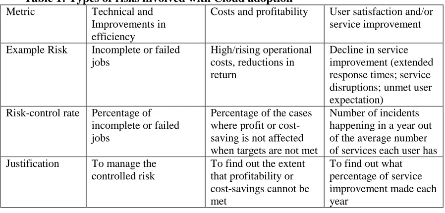
OSM is generally used in three areas: technical, cost and user (or client) satisfaction before and after deploying the new solution. However, since each system adoption is unique as are their precise objectives, suitable metrics should be defined for each. These metrics are summarised in Table 1. For example:
Technical: Efficiency gains may be measured by consideration of the completion times for Cloud and non-Cloud systems times. The risk-control rate is given by the proportion of failed requests/tasks.
Cost: Data will need to be collected regarding costs or profitability improvements arising from introducing new technology and the risk-control rate is the rate of gain assured even when targets are not met.
[image:7.612.84.533.509.724.2]Users: Quality of service improvements which are usually evaluated from periodic user surveys. The risk-control rate reflects the rate at which incidents happen.
Table 1: Types of risks involved with Cloud adoption Metric Technical and
Improvements in efficiency
Costs and profitability User satisfaction and/or service improvement
Example Risk Incomplete or failed jobs
High/rising operational costs, reductions in return
Decline in service improvement (extended response times; service disruptions; unmet user expectation)
Risk-control rate Percentage of incomplete or failed jobs
Percentage of the cases where profit or cost-saving is not affected when targets are not met
Number of incidents happening in a year out of the average number of services each user has Justification To manage the
controlled risk
To find out the extent that profitability or cost-savings cannot be met
3.1 OSM datasets processing
Metrics collection can be undertaken by system automation or by surveys. Hundreds or thousands of datasets can be collected in this way while running experiments or conducting surveys over a period of time. This will ensure large sample sizes for modelling although numerous datasets makes analysis more complex and time consuming (Huson et al., 2007).
The data for the following experiments are taken from our previous work (Chang et al., 2013), which involved daily backup of thousands of medical files and experimental data at a National Health Service involving a total of 10 petabytes of data (Chang and Ramachandran, 2016). Each file contains thousands of records of patient or medical data including tumour, DNAs, proteins and images (Chang et al., 2013). Each backup operation generated records of information linked to each file, which contains thousands of datasets. The relationship between datasets and datapoints is as follows. Each dataset contains up to 2,000 rows and 255 fields of records, equivalent to 510,000 datapoints. There are 500 datasets involved, which becomes 500 x 510,000 = 255,000,000 datapoints for analysis. OSM is able to process 255,000,000 datapoints in seconds. The capacity of processing such a large number of datapoints in seconds is important for Big Data analysis and businesses (Huson et al., 2007).
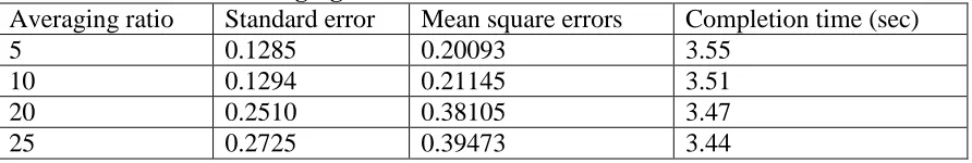
[image:8.612.100.546.553.628.2]Gardner and Altman (1986) explain a technique in which they filter data sets to remove outliers and then repeat their statistical analysis thereby improving data quality and accuracy of results. OSM uses a similar technique collecting datasets into averaged groups before analysis. The averaging ratio is used to optimise the performance in dataset processing. Our previous work shows that it can shorten the execution time of job completion for dataset processing (Chang, 2014 a). The averaging ratio is commonly a multiple of 5 and depends on the size of the datasets. For smaller sets (under 1,000 datasets), the averaging ratio used is 5, rising to 20 for datasets in excess of 6000. Results of a series of experiments showing the effect of using various averaging ratios when using 500 datasets are shown in Table 2 and confirm that the averaging ratio should be small for small datasets.
Table 2: Results of averaging ratios for 500 datasets
Averaging ratio Standard error Mean square errors Completion time (sec)
5 0.1285 0.20093 3.55
10 0.1294 0.21145 3.51
20 0.2510 0.38105 3.47
25 0.2725 0.39473 3.44
3.2 OSM outputs
Statistical modelling in OSM uses multiple observations of a, e and rc as the inputs to compute risk. Outputs will include the following:
Beta (β), a measure of uncontrolled risk that may affect the project.
Standard Error of the mean: the range of the mean of the experimental results. Smaller standard errors imply more accurate and representative results.
Durbin-Watson (1950, 1951), a test to detect autocorrelation (a relationship between values separated from each other by a given time lag) in the residuals of a regression analysis. Durbin-Watson results should be >1 (Hull, 2009; Lee et al., 2010).
Durbin-Watson is applied to regression computed by OSM. The value for Pr > DW corresponds to the negative autocorrelation test (residuals eventually wither off), which means the difference between the expected and actual values becomes small and even negligible if the OSM is running continuously. Thus, the negative autocorrelation test is a preferred method in the OSM approach. The value of Pr > DW should ideally get close to 1 to reflect the accuracy of the OSM regression. The difference between 1 and Pr > DW gives the p-value for the OSM analysis.
Additional OSM outputs provide more information about beta and regression accuracy:
Mean Square Error (MSE) is an estimator to quantify the difference between estimated and actual values. A low MSE value means there is a high correlation between actual and expected return values.
R-squared values: There are two interpretations for R-square. Firstly, R-Squared value indicates how good a fit the regression line is to all the datapoints. In other words, how close the actual result is to the theoretically desirable values. Samson and Terziovski (1999) assert that the value of regression R-square should be close to 1 if the emphasis is on prediction. The value may be lower if the focus is to study the relationship between input variables, but additional explanations should be provided. Although OSM is not a predictive model and it studies relationships between three key inputs, the regression R-square (99.99% confidence interval, C.I) is used to describe how well a regression line fits a set of data. If the result is below 0.5, another regression with 95% C.I (with both upper and lower limit) is required.
and the R-squared value provides a good indication for the percentage and sources of beta risks.
3.3 Performance comparison between CAPM and OSM: Single job comparison
Traditional CAPM struggles to work with thousands of datasets at once. It is not a computing problem but a design problem, since the model is originally designed to compute risk and return calculations with less regard to the quantity of datasets (Pretcher and Parker, 2007; Hey et al., 2009). Attempts have been made to design improved models which allow processing of large volume of datasets at once but work published by researchers focus on the quantitative analysis without presenting the algorithm. In addition their techniques require the data to be reorganised before CAPM data processing can begin which adds to the computational burden.
These comparisons were performed on three platforms:
A desktop environment with a 2.67 GHz Intel Xeon Quad Core processor and with 12 GB of memory installed of which 4 GB was allocated to each of two virtual machines.
A private Cloud using VMware VSphere 4 with Virtual servers running supported by 1 gigabyte per second (GBp/s) network connections. Each of the 16 nodes has an AMD Opteron 6200 running at 3.4GHz along with 16GB of RAM, bringing the total hardware capability to 24.2 GHz and 32 GB RAM.
An Amazon EC2 public cloud with quad core CPUs, running at 2.33 GHz and with 4 GB of memory.
The purpose of this experiment was to compare performance on desktop, a private cloud and a public cloud for a single job request which entails processing 2,000 datasets, each of which containing thousands of datapoints. The computational work is to ensure that both key inputs in CAPM and OSM can be processed with key outputs produced. These key output values contain beta, standard error and Durbin-Watson for both OSM and CAPM. All key outputs should be identical. The tasks include:
- Completion of processing all datasets for CAPM and OSM.
- Data processing to produce key outputs and comparison of execution times for job completion.
All the single jobs for OSM and CAPM data processing should be completed
Key outputs must be identical
If these conditions are not met, the conditions for performance comparisons are not valid, and experiments need to be repeated. In all the experiments, all the data processing results satisfy these two conditions.
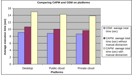
Table 3: Total time for running CAPM and OSM data processing on three different platforms with 95% confidence level
CAPM: average total time (sec) without manual extraction CAPM: average total time (sec) with manual extraction OSM: average total time (sec) Performance improvement (OSM vs. CAPM without manual extraction) Performance improvement (OSM vs. CAPM with manual extraction) Output results Same results?
Desktop 10.68 15.02 9.08 OSM is 14.98% better OSM is 39.55% better β = 0.4509 SE = 0.1111 DW = 1.2259 Yes Public cloud
10.04 14.31 8.85 OSM is
11.85% better OSM is 38.16% better β = 0.4509 SE = 0.1111 DW = 1.2259 Yes Private cloud
9.63 13.86 8.67 OSM is
9.97% better OSM is 37.45% better β = 0.4509 SE = 0.1111 DW = 1.2259 Yes
There is a significant performance improvement comparing OSM and CAPM with manual extraction in Table 3. The improvement is 39.55% better on desktop, 38.16% on a public cloud and 37.45%, on a private cloud. Although performance between OSM and CAPM is only between 4 and 6 seconds faster, the difference in the actual performance is significant when the number of datasets processed per day is taken into account. This translates into a time-saving of up to 40% to complete processing of all large datasets as demonstrated in a further set of experiments described in Section 3.4.
same results. Although the desktop has the highest percentage performance improvement, the execution time is the shortest for the private cloud followed by public cloud and then desktop. Multiplatform tests were undertaken to ensure that OSM can work across platforms efficiently.
Comparing CAPM and OSM on platforms
0 2 4 6 8 10 12 14 16
Desktop Public cloud Private cloud
Platforms
A
v
e
ra
ge
e
x
e
c
ut
ion
t
im
e
(
s
e
c
)
OSM: average total time (sec)
[image:12.612.107.542.144.396.2]CAPM: average total time (sec) without manual distraction CAPM: average total time (sec) with manual distraction
Figure 1: CAPM and OSM performance comparisons on three different platforms
3.4 Performance comparison between CAPM and OSM: processing thousands of datasets containing millions of datapoints
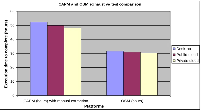
Many datasets are analysed in real-time and performance improvement is useful to ensure a smooth trading process throughout the daily trading period. The objective for the exhaustive test is to allow a large volume of data (each containing 2,000 datasets) to be processed simultaneously and then to find out the difference between OSM and CAPM completion time. Although there is only 6 second difference per job, the difference would vary significantly while processing thousands of jobs, which means processing thousands of datasets for thousands of times.
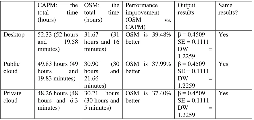
time taken by OSM and CAPM to process this data was measured on each of the three platforms. The results are shown in Table 4 and Figure 2.
Table 4: Total time for running CAPM and OSM models (exhaustive and automated tests)
CAPM: the total time (hours)
OSM: the total time (hours)
Performance improvement
(OSM vs.
CAPM)
Output results
Same results?
Desktop 52.33 (52 hours and 19.58 minutes)
31.67 (31 hours and 16 minutes)
OSM is 39.48% better
β = 0.4509 SE = 0.1111
DW =
1.2259
Yes
Public cloud
49.83 hours (49 hours and 19.83 minutes)
30.90 (30 hours and 21.66
minutes)
OSM is 37.99% better
β = 0.4509 SE = 0.1111
DW =
1.2259
Yes
Private cloud
48.26 hours (48 hours and 6.3 minutes)
30.21 hours (30 hours and 5 minutes)
OSM is 37.40% better
β = 0.4509 SE = 0.1111
DW =
1.2259
Yes
[image:13.612.84.526.139.348.2]CAPM and OSM exhaustive test comparison 0 10 20 30 40 50 60
CAPM (hours) with manual extraction OSM (hours)
[image:14.612.112.525.73.300.2]Platforms E x e c u ti o n t im e t o c o m p le te ( h o u rs ) Desktop Public cloud Private cloud
Figure 2: CAPM and OSM performance comparisons
Table 5: Other comparisons between traditional CAPM and OSM data processing
Other comparisons Traditional CAPM OSM
Suitability for Cloud Computing, including risk and return analysis
This is a generic model for many areas but not designed for risk and return analysis of Cloud adoption
This is an improved method suitable for Cloud adoption, particularly risk and return analysis Large volume of datasets Less capable of handling Large
volume of datasets. Need procedures or steps to process
Better to handle volume of large datasets
Performance Lower performance Relative better performance Handling of complex data Needs manual extraction for
further analysis. It can take a long time depending on complexity.
Presents all analysed data as 3D visualisation to exploit complex data. It also allows stakeholders to understand data analysis more easily
Results in our experiments show that OSM can complete the data processing of 2,000 datasets more quickly than the traditional model and it removes the need for manual extraction. In the exhaustive test, the advantage of using OSM is illustrated by saving the data processing time of 20 hours. Four additional areas of comparison: (i) Suitability for Cloud Computing; (ii) Large volume of datasets; (iii) Performance and (iv) Handling of complex data are presented in Table 5. Analysis of comparisons is supported by results presented in Sections 3, 4, 5 and 6.
4 Case Study 1: The iSolutions Group, the University of Southampton
staff. The purpose is to identify the level of service improvement evaluated by users. They have been recording user feedback and ratings since 2008.
Three years of data between 2008 and 2011 was obtained to study service improvement, which is an important factor for supporting good system design, deployment and services including Cloud Computing (Chowhan and Saxena, 2011). The 2008/2009 survey gave management the ideas of what they were to measure and identification of important areas for service improvement. In other words, their 2009/2010 and 2010/2011 surveys were focused on key areas of service improvement and the use of OSM to select datasets suitable for analysis and interpretation of results.
This case study considers users’ evaluation in four areas defined by Corporate Planning and the iSolutions Group of the University of Southampton:
Accessibility
Adequacy of financial support
Availability
Sufficiency of support
Survey is used as a research method to understand how users evaluate Cloud services annually. To address these four areas, four main questions were used. Each user is asked to provide a score from 0 to 10, (where 0 means no service at all and 10 means the service was perfect) against each of the following statements:
I have adequate access to the equipment necessary for my research (Accessibility)
There is appropriate financial support for research activities (Adequacy of financial support)
There is adequate provision of computing resources and facilities (Availability)
I have the technical support I need (Sufficiency of support)
Since an important objective is to understand the service improvement before and after service adoption, investigations over a substantial period of time are relevant and useful to the final analysis. Instead of undertaking the survey for one year, the same questions were asked annually throughout 2009 to 2011. This allows stakeholders to monitor the yearly rating evaluated by users and identify areas for improvements each year. To meet OSM requirements, the expected scores were taken one year before the following survey. The breakdown of the survey is as follows.
Year 2009: expected scores for 2010 only.
Year 2010: expected scores for 2010 and actual scores for 2009.
Year 2011: expected scores for 2012 and actual scores for 2011
All the users were asked to give a current actual score and an expected score for the following year each time they took the survey.
4.1 The OSM metrics
Expected service rating is the expected return value for OSM. The average of four ratings (accessibility, finance, availability and support) per user is the expected score for each user.
Actual service rating is the actual return value for OSM from the survey. The average of their four ratings is the actual score for each user.
Risk-control rate: Users were asked to give the number of incidents which happened in 2009/2010 and 2010/2011. The risk-control rate is taken to be this number divided by 200 which is iSolutions Group’s estimate of the average number of requests per user each year.
The service improvement is the difference between each comparison every year. Comparison of the same users’ feedback every year should ensure risk-control rates vary by no more than 0.5% throughout the period of survey since risk-control rates which vary significantly have undesirable impacts on the quality of analysis. Comparison between 2009-2010 and 2010-2011 services is the difference between 2009-2010 and 2010-2011 score values for each user, which is equivalent to the rate of service improvement.
The criteria used to select valid data entries were as follows:
Selected users must answer all questions.
Users need to have experience of using and receiving the services in 2009/2010 and 2010/2011 each year for a minimum of 60 hours a year.
These data quality requirements meant only 200 entries qualified for the OSM analysis.
4.2 Key OSM outputs
Computational modelling of OSM used a, e, rc as the input to compute risk. The outputs included the following:
1. Beta (β) is the value determining the risk measure (or the extent of the volatility), the uncontrolled risk.
2. Standard Error (SE) of the mean, the range of the mean that the experimental results fall into for OSM. The smaller the standard error, the smaller the difference between expected and actual return values.
4. Mean Square Error (MSE), an estimator to quantify the difference between estimated and actual values. A low MSE value means there is a high correlation between actual and expected return values.
5. R-squared value which is used to determine the regression fits the data. Both 95% and 99.99% Confidence intervals (CI) are computed. In this context, it is referred as “R-squared value for firm”, a term commonly used in econometrics to describe the percentage of risks in proportion to the external or internal organizations or factors. If an organization has an R-squared value (99.99 C.I) of 0.3, this means 30% of risks are from external bodies or the market and 70% of risks come from the organization such as poor adoption decision, overspending, poor selection of equipment, etc.
4.3 The OSM results and analysis
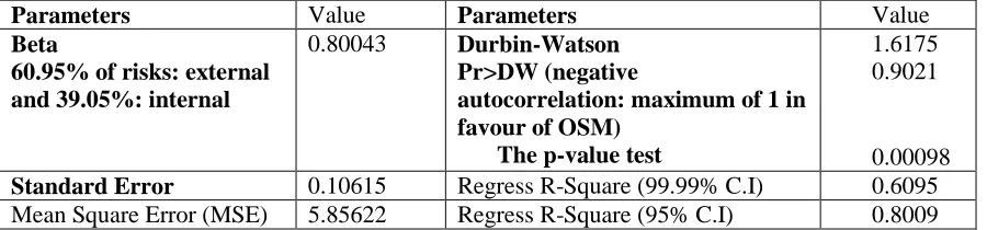
[image:17.612.85.535.317.422.2]Results of OSM case study 1 are shown in Table 6.
Table 6: OSM Case 1 for service improvement of the iSolutions, University of Southampton
Parameters Value Parameters Value
Beta
60.95% of risks: external and 39.05%: internal
0.80043 Durbin-Watson Pr>DW (negative
autocorrelation: maximum of 1 in favour of OSM)
The p-value test
1.6175 0.9021
0.00098
Standard Error 0.10615 Regress R-Square (99.99% C.I) 0.6095 Mean Square Error (MSE) 5.85622 Regress R-Square (95% C.I) 0.8009
Interpretation of the three key statistics:
Beta is equal to 0.80043. This is a medium-high value since it is still below 1. The project itself has a medium-high volatility of uncontrolled risks. This means current levels of user satisfaction are divided. Although most of the users acknowledged the usefulness of Cloud services, some provided feedback that there was still room for improvement. The variation between users’ opinions also suggested that the management should take continuous service improvement more proactively.
Standard error is 0.10615 and is relatively low, which suggests there is extremely high consistency between all metrics with very few outliers.
The first order Durbin-Watson result shows that there is a high negative autocorrelation (0.9021) favouring OSM, which means a good quality of data and standard errors. The p-value test result is 0.00098 and is also acceptable.
In addition:
10% and 20% expected and actual rate of improvement. The third group consists of about 10% of the sample population and they have a higher expected rate of improvement than the actual rate, although both rates are positive. It is important to find out any reasons behind their scores and interviews with users should be undertaken before their next survey.
Regression R-square is 0.6095 and it is optional to use 95% C.I to analyse. Regression with 95%. C.I is 0.8009, which means all data fits well with regression. This means 60.95% risks are from external such as status in funding and change of policy due to the change of Vice Chancellor. 39.95% of risks are from internal such as lack of training for staff and users.
5 Case Study 2: The University of Greenwich in adopting supply chain Cloud
This case investigated user evaluation of a new Cloud service, supply chain Cloud, in teaching and learning activities. Chang and Wills (2013) report that the use of Private Cloud applications helps improve students’ learning satisfaction. This case study was undertaken together with Chang and Wills’ (2013) study to review the Year 2012 user evaluation. Unlike Case Study 1, this case study does not keep track of every user, because the University of Greenwich (UoG) adopts a different operational model that different cohort groups are used for learning activities each year. Despite this, OSM is able to provide relevant metrics and offer analysis of user evaluation of Year 2012 data.
To make OSM a model suitable for UoG, two cohort groups of students were used for this case who had followed the supply chain learning for six months. Cohort group one had 16 learners and cohort group two had 23 learners. Each learner wrote scores for learning satisfaction before the adoption of supply chain Cloud. They attended the learning workshops at least two hours a week in a classroom environment and additional hours for learning. User evaluation was taken before the end of the delivery of the six-month learning period, contributing to the final user evaluation score. All the user evaluation scores were taken and compared with each cohort group.
5.1 The OSM metrics overview
The OSM metrics are recorded and presented as follows:
The expected learning satisfaction was recorded prior the use of the supply chain Cloud.
The actual learning satisfaction was recorded after the use of the supply chain Cloud.
altogether a maximum of 50 cases of complaints can be accommodated as the risk-control rate. All these complaints had to be resolved as soon as possible.
Two cohort groups took part in this study. Data collected was used for their analysis. The management decided that each cohort group should have their results of analysis.
5.2 The OSM results and analysis
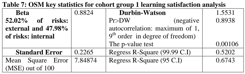
[image:19.612.104.530.223.353.2]This section shows the results of OSM analysis for both cohort groups. Table 7 shows results for cohort group 1.
Table 7: OSM key statistics for cohort group 1 learning satisfaction analysis Beta
52.02% of risks: external and 47.98% of risks: internal
0.8824 Durbin-Watson
Pr>DW (negative
autocorrelation: maximum of 1, 9th order in degree of freedom) The p-value test
1.5531 0.8938
0.00106
Standard Error 0.2265 Regress R-Square (99.99 C.I) 0.5202 Mean Square Error
(MSE) out of 100
7.84874 Regress R-Square (95 C.I) 0.6743
Further explanations are presented as follows:
Beta is equal to 0.8824. The medium-high value suggests the project risk is maintained at an acceptable but subject to a high risk. A likely reason is that although all users acknowledge the positive learning experience, a number of them only acknowledge 11-13% improvement against the average of 15% improvement.
Standard error is 0.2265. The low value suggests most metrics are close to each other and the data has few extremes. There is high consistency between all metrics.
The ninth order Durbin-Watson: Pr > DW is the p-value for testing negative auto-correlation which favours OSM. Results show that there is a high negative auto-correlation (0.8938). The 9th order means the Durbin-Watson test is calculated nine times to get the closest value to the recommended p-value, which is 0.00106 and slightly above the recommended 0.0010. A likely reason is because of a wider variation in the improvement of feedback. Some only gave 11% more improvement and a few gave 17% and above.
The Mean Square Error (MSE) value is 7.84874. However, it is considered a low value out of 100, since all ratings are presented out of 100 rather than the typical out of 1.
learning difficulties. They acknowledged the improved learning satisfaction, but they provided feedback that some part of the course was not easy to understand.
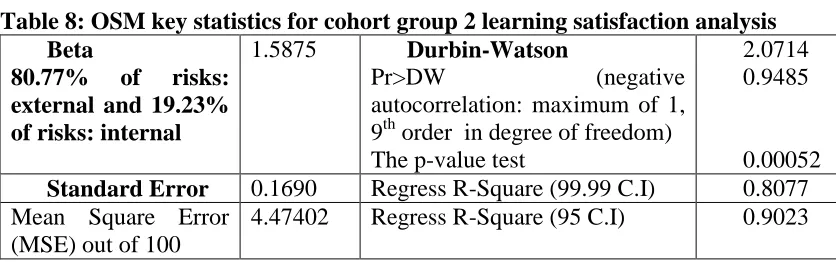
[image:20.612.108.526.122.253.2]Table 8 shows results for the cohort group 2.
Table 8: OSM key statistics for cohort group 2 learning satisfaction analysis Beta
80.77% of risks: external and 19.23% of risks: internal
1.5875 Durbin-Watson
Pr>DW (negative
autocorrelation: maximum of 1, 9th order in degree of freedom) The p-value test
2.0714 0.9485
0.00052
Standard Error 0.1690 Regress R-Square (99.99 C.I) 0.8077 Mean Square Error
(MSE) out of 100
4.47402 Regress R-Square (95 C.I) 0.9023
Further explanations are presented as follows.
Beta is equal to 1.5875. The high value suggests the project risk is high. However, there is a different reason for this. Group 2 felt the delivery exceeded their expectations and provided positive feedback. Their expectations for the following years were exceptionally high, which some services were unable to match or had to be re-negotiated with the expected delivery for the following year. It was their overwhelming opinion that realistic goals should be set, negotiated and agreed before the following delivery.
Standard error is 0.1690. The low value suggests most metrics are close to each other and the data has fewer extremes. There is a high consistency between all metrics.
The second order Durbin-Watson: Pr > DW is the p-value for testing negative auto-correlation which favours OSM. Results show that there is a high negative auto-correlation (0.8938). The 2nd order means the Durbin-Watson test is calculated a second time to get the closest value to the recommended p-value, which is 0.00515. The Durbin-Watson value is 2.0714 and is an acceptable value.
The Mean Square Error (MSE) value is 4.47402. However, it is considered a low value out of 100, since all ratings are presented out of 100 rather than the typical out of 1.
Main regression R-square is 0.8077 which means 80.77% of the risks are from the externals such as the type of the course that learners must pick this course. 19.23% of the risks are from the internals, which include that some learners struggled at some stage of learning but eventually they overcame learning difficulties. Comparing to group 1, group 2 had more positive views for learning.
6 Discussion
This section presents four topics for discussions. The first topic is the use of OSM for advanced analysis such as visualisation. Visualisation for two case studies is presented in this section. The second topic is the general discussion of OSM and the third topic is the comparison with similar models for Cloud Computing. The last topic concludes how OSM is a justifiable Emerging Service and Analytics in Cloud Computing.
6.1 The OSM results and analysis
The purpose is to present complex analysis in a format that stakeholders and reviewers without statistical or computing backgrounds can understand. The use of visualisation is crucial to the development of the organisation’s business intelligence strategy that can blend their business processes with the use of Cloud Computing services (Chang et al., 2011 a; 2011 b; Chang, 2014 b). OSM can provide additional services such as Visualisation. The OSM metrics, actual return values, expected return values and risk-controlled rate of two case studies may be presented as follows.
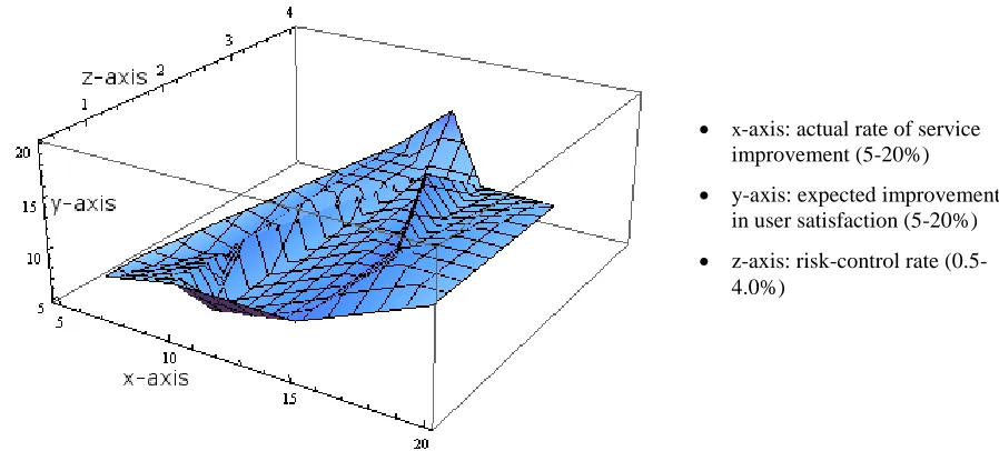
6.1.1 Visualisation for Case Study 1
Figure 3 shows Visualisation for the iSolutions Group of the first OSM case study. The x-axis reflects an actual rate of service improvement between 5% and 20%. The y-axis reflects expected rate of service improvement between 5% and 20%. The z-axis shows risk-control rate between 0.8% and 4.4%. The shape in the 3D Visualisation can indicate the status of the project (Chang et al., 2011; Chang, 2014 a, 2014 b). Spikes and bumps indicate variations or volatility experienced in the project. The OSM formula suggests that the correlation between all these three metrics is important to keep a high consistency between all metrics. The majority of the metrics in Figure 3 is aligned with each other with only a few spikes experienced in the figure.
Figure 3: Visualisation for the iSolutions Group’s Cloud service improvement, University of Southampton
x-axis: actual rate of service improvement (5-20%)
y-axis: expected improvement in user satisfaction (5-20%) z-axis: risk-control rate
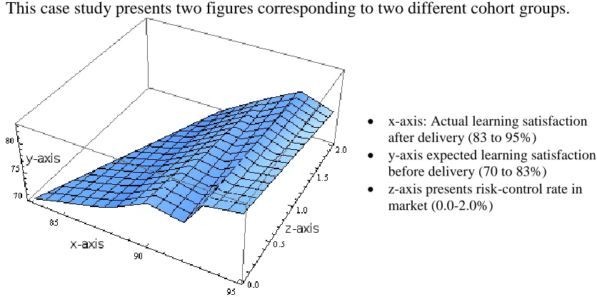
[image:21.612.101.550.481.684.2]6.1.2 Visualisation for Case Study 2
This case study presents two figures corresponding to two different cohort groups.
Figure 4: Visualisation for learning satisfaction of using supply chain Cloud, cohort group 1, University of Greenwich (UoG)
Figure 4 shows Visualisation for the cohort group 1 of the third OSM case study. The x-axis reflects the actual learning satisfaction after Cloud teaching delivery between 83% and 95%. The y-axis reflects the expected learning satisfaction before Cloud teaching delivery between 70% and 83%. The z-axis shows risk-control rate between 0% and 2%. The shape in Visualisation suggests that some learners were towards the lower end of learning satisfaction before the delivery, and they moved to the higher end of learning satisfaction after the delivery. Some of them provided feedback that the use of supply chain Cloud for their learning was a new experience with a steep learning curve, they were happy to overcome the learning challenge.
Figure 5: Visualisation for learning satisfaction of using supply chain Cloud, cohort group 2, University of Greenwich (UoG)
x-axis: Actual learning satisfaction after delivery (83 to 95%)
y-axis expected learning satisfaction before delivery (70 to 83%) z-axis presents risk-control rate in
market (0.0-2.0%)
x-axis: Actual learning satisfaction after delivery (88 to 96%)
y-axis expected learning satisfaction before delivery (72 to 86%) z-axis presents risk-control rate in
[image:22.612.104.522.101.309.2] [image:22.612.101.539.488.682.2]Figure 5 shows Visualisation for the cohort group 2 of the third OSM case study. The x-axis reflects the actual learning satisfaction after Cloud teaching delivery between 88% and 96%. The y-axis reflects the expected learning satisfaction before Cloud teaching delivery between 70% and 83%. The z-axis shows risk-control rate between 0% and 2%. The shape suggests that the majority of learners had perceived the positive learning experience and the extent of the increased learning satisfaction after the delivery was more in proportion than group 1. However, the high learning satisfaction after the delivery made them set higher expected goals for the next delivery. This also means that service level agreements (SLA) should be renegotiated and revised with users.
6.2 General discussions of OSM and comparisons with similar models
This section presents discussion about OSM and comparisons with similar models. Compared with CAPM which was not designed to handle huge datasets and is not designed for analysis of system adoption such as Cloud Computing, OSM has an improved methodology and formula. OSM can compute thousands of datasets at once and is designed for Computing (including Cloud Computing) rather than as a generic model for risk and return. Referred to Section 3, comparisons between OSM and CAPM show OSM has a better performance than CAPM both in a test of processing 2,000 datasets and in an exhaustive test. While identifying and collecting metrics for actual return values, expected return values, risk-control rates, OSM can calculate key values including beta, standard error and Durbin-Watson (with negative autocorrelation) to interpret the collected datasets.
A Cloud Computing project with satisfactory outcomes should have the following:
Low beta: low uncontrolled risk.
Low standard error: Results of collected datasets are highly consistent.
Durbin-Watson value above 1, and negative autocorrelation test is as close as to 1 as possible. The p-value should be below 0.001.
R-squared values, used to identify proportions and sources of beta risks should be above 0.5 and below 1.
Mean Squared values and positive p-values should have low values to support accuracy of OSM analysis.
6.3 Comparisons with similar models
This section is focused on a comparison between OSM, CAPM and similar models, particularly the two models mentioned in Section 2, which aim to make scholarly contributions by demonstrating improved models in economics that can be used in Cloud Computing. The criteria for comparison are:
1. The analysis of risk and return status of the Cloud Computing adoption: The proposed method should address general issues and widen scope beyond risk and return (Sharma et al., 2012). Return is not limited to profits but can include user satisfaction and other perspectives. Risk is not limited to security but a greater coverage of risk assessment (Sharpe, 1992; Harland, 2003).
2. Dividing risks into uncontrolled and managed status: Following the essence of Capital Asset Pricing Model (CAPM) (Markowitz, 1952; Lintner, 1965 a, 1965 b; Mossin, 1966; French, 2003) and the Nobel lecture given by William Sharpe (1964, 1992), all risks are divided into uncontrolled and managed status.
Additionally, it should offer measurement in regard to “free rate” or risk-control rate while dividing risk into managed and unmanaged categories. The proposed model should have guidelines and scientific or systematic processes for measuring the “risk-free rate. It should be based on the users’ perspective. If it is defined by the service provider, it should be based on the number of accidents or complaints made by users.
3. Handling of large data: The proposed model should be able to process large quantities of datasets and large numbers of datapoints in the datasets (Dean and Ghemawat, 2008). Requirements for performance and accuracy should be met. 4. Case studies: The proposed model should have case studies to demonstrate that it
is usable beyond the theoretical framework (Khajeh-Hosseini et al., 2010; Han, 2011).
OSM is already supported by several case studies, including:
Vodafone and Apple (Chang et al., 2011 a): OSM was used to analyse the profitability and risk. There was an actual 21-26% gain in the profitability after adopting Mobile and Cloud services.
SAP (Chang et al., 2011 a): OSM was used to analyse the effectiveness of using SAP for small and medium enterprises (SMEs) to manage their risks within 1%. OSM helps to clarify how SMEs could withstand the impact due to financial crisis.
National Health Service (NHS) (Chang et al., 2011 b): The status of risk and return of two NHS projects has been evaluated by OSM. The outputs provided useful information for the stakeholders.
Table 9: Comparisons between OSM, CAPM, Sharma et al. and Quanbari et al.
Models and criteria Generic risk and return definition and analysis
Uncontrolled and managed risk division (and measurement of risk-free/risk-control rates)
Handling of large data
Case studies
CAPM (Markowitz, 1952; Sharpe, 1964, 1992; Lintner, 1965 a, 1965 b; Mossin, 1966; French, 2003)
It provides a generic model to measure and analyse risk and return.
The model divides risk into uncontrolled (beta) and managed (risk-free rate). But criticism is drawn on unscientific definition of risk-free rate.
It is not designed for this at all.
There are case studies but the majority of them are in economics and finance.
Sharma et al. (2012) Their approach is developed on Black Scholes Model (BSM) which deals with risk and return on investment. Their focus is on the service providers.
There is no consideration in dividing risk into uncontrolled and managed. Their proposal suggests following their steps, risks are all managed.
It is not designed for this, even though they
have experiments
showing they can deal with Service Level Agreement agenda.
No there yet.
Quanbari et al. (2014)
Their approach is
developed on Binomial Tree which studies dependencies within risk, or return.
There is no consideration in dividing risk into uncontrolled and managed.
It is not designed for this.
No there yet.
OSM (Chang et al., 2011 a; 2011 b; 2012)
OSM deals with the risk and return status, analysis and review of services and project that adopt Cloud Computing. User satisfaction is inclusive.
The model divides risk into uncontrolled (beta) and managed (risk-control rate). There are definitions on how to measure the manage risk which also take users into considerations.
OSM can handle
thousands of datasets, millions of datapoints and compute them a single job in seconds and thousands of jobs in hours demonstrated in Section 4.
OSM has several case studies to support the validity of the model.
Additional case
studies were
6.4 OSM as an Emerging Service and Analytics
Emerging Services and Analytics provide a unique service for Cloud Computing, since it combines the state-of-the-art of the system design and implementation, technology integration and business models for Platform as a Service (PaaS) and Software as a Service (SaaS). Examples include services and analytics for healthcare, finance, education, mobile services, transportation, energy, natural science and physical science. Emerging Services and Analytics workshops have been successfully delivered to demonstrate the research contributions and case studies in this area (Chang et al., 2014, 2015). An emerging model to analyse Cloud Computing projects, process a large number of data and interpret the outputs in a way that enables the stakeholders to understand is essential for the development of Cloud Computing.
OSM is an Emerging Service and Analytics, which provides added value for users and organisations adopting Cloud Computing. Firstly, OSM defines and interprets the status of risk and return for Cloud Computing projects. Return can be in the form of technical, cost and users’ focuses in Cloud Computing. Examples and computations for risk-control rate and uncontrolled risk (beta) have been presented. Secondly, OSM can process thousands of datasets at once and is specifically designed for a large data processing and analytics. Thirdly, OSM performs much better than a comparative model, CAPM, under the same experimental conditions. Fourthly, interpretations and data analysis computed by OSM can explain the overall status of the projects, the extents of risks and their detailed implications. Fifthly, visualisation can help the stakeholders to understand the actual rate of return, expected rate of return and risk-control rate of their project without the need to check all the datasets. Sixthly, there are two case studies to confirm that OSM is useful for organisations adopting Cloud Computing. Lastly, OSM provides more in-depth information, metrics, qualitative and quantitative analysis and recommendations than other similar approaches.
7 Conclusion
for econometrics at a time when datasets were much smaller than is common today. We therefore propose OSM which is based on CAPM but has been tuned to match the particular requirements of an organisation adopting Cloud Computing. OSM produces more accurate results and comfortably out performs CAPM when analysing substantial datasets. OSM provides an emerging service and analytics model to ensure technical, costs and profitability and user satisfaction can be modelled and computed according to different organisational requirements for Cloud Computing adoption.
The case for OSM is illustrated by two case studies confirming and supporting the validity and effectiveness of OSM. Outputs are useful for analysis. OSM has met four criteria for evaluation of Cloud Computing adoption and thus is a suitable emerging service and analytics model for Cloud Computing.
8 References
Agopyan, A., Sener, E., Beklen, A., Financial Business Cloud for High-Frequency Trading, International Journal On Advances in Intelligent Systems, 4 (2011) 203-217.
Chang, V., De Roure, D., Wills, G., Walters, R. J. Case studies and organisational sustainability modelling presented by Cloud Computing Business Framework. International Journal of Web Services Research, 8(3), (2011), 26-53.
Chang, V., De Roure, D., Wills, G., Walters, R. J., Barry, T. Organisational Sustainability Modelling for Return on Investment (ROI): Case Studies Presented by a National Health Service (NHS) Trust UK. CIT. Journal of Computing and Information Technology, 19(3), (2011), 177-192.
Chang, V., Wills, G., Walters R. J., and Currie, W., Towards a structured Cloud ROI: The University of Southampton cost-saving and user satisfaction case studies. In Sustainable ICTs and Management Systems for Green Computing., IGI Global, (2012), 179-200.
Chang, V., Wills, G., A University of Greenwich Case Study of Cloud Computing. E-Logistics and E-Supply Chain Management: Applications for Evolving Business, (2013), 232-245.
Chang, V., Walters, R.J., Wills, G., Cloud Storage and Bioinformatics in a private cloud deployment: Lessons for Data Intensive research. In, Cloud Computing and Service Science., Springer Lecture Notes Series, Springer Book, 2013.
Chang, V., A proposed model to analyse risk and return for Cloud adoption. Lambert Academic Publishing, (2014 a), 316 pp.
Chang, V., The business intelligence as a service in the cloud. Future Generation Computer Systems, 37, (2014 b), 512-534.
Chang, V., A proposed Cloud Computing Business Framework. Nova Science Publisher, (2015 a).
Chang, V., Chang, V., Towards a Big Data System Disaster Recovery in a Private Cloud. Ad Hoc Networks, (2015 b), in press.
Chang, V., Wills, G., & Walters, R. J. (2014). ESaaSA 2014-Proceedings of the International Workshop on Emerging Software as a Service and Analytics.
Chang, V., Ramachandran, M., Wills, G., Walters, R. J., Kantere, V., & Li, C. S. (2015). ESaaSA 2015-Proceedings of the International Workshop on Emerging Software as a Service and Analytics, Lisbon, Portugal, May 20-22, 2015.
Chowhan, S. S., Saxena, R., Customer Relationship Management from the Business Strategy Perspective with the Application of Cloud Computing, Proceedings of DYNAA 2011 workshop, 2(1), (2011), Oct.
Damodaran, A., Dealing with Risk: Investment Analysis, Lecture Notes, Chapter 4, New York University Business School, 2008.
Dean, J., & Ghemawat, S. MapReduce: simplified data processing on large clusters. Communications of the ACM, 51(1), 2008, 107-113.
Durbin, J., G.S. Watson, G.S., Testing for Serial Correlation in Least Squares Regression: I, Biometrika, 37(3-4), 1950, 409-428.
Durbin, J., G.S. Watson, G.S., Testing for Serial Correlation in Least Squares Regression. II, Biometrika, 38 (1951) 159-177.
French, C.W., The Treynor Capital Asset Pricing Model, Journal of Investment Management, 1 (2003) 60-72.
Gardner, M.J., D.G. Altman, D.G., Confidence-Intervals Rather Than P-Values - Estimation Rather Than Hypothesis-Testing, Brit Med J, 292 (1986) 746-750.
Hamelink, F., Optimal international diversification: Theory and practice from a Swiss investor's perspective, FAME, 2000.
Hammond, M., Hawtin, R., Gillam, L., Oppenheim, C., Cloud Computing for Research, in, JISC, 2010.
Han, Y. Cloud computing: case studies and total cost of ownership. Information technology and libraries, 30(4), 2011, 198-206.
Harland, C., Brenchley, R., & Walker, H. Risk in supply networks. Journal of Purchasing and Supply management, 9(2), (2003), 51-62.
Hey, A.J.G., Tansley, S., Tolle, K., The fourth paradigm: data-intensive scientific discovery, in, Microsoft Research, Redmond, USA, (2009).
Hull, J.C., Options, Futures, and Other Derivatives, Seventh Edition ed., Pearson, Prentice Hall, 2009.
Huson, D.H., Auch, A.F., Qi, J., Schuster, S.C., MEGAN analysis of metagenomic data, Genome Res, 17(3), (2007), 377-386.
Jiang, P., & Rosenbloom, B. Customer intention to return online: price perception, attribute-level performance, and satisfaction unfolding over time. European Journal of Marketing, 39(1/2), (2005), 150-174.
Iosup, A., Ostermann, S., Yigitbasi, M. N., Prodan, R., Fahringer, T., Epema, D. H., Performance analysis of cloud computing services for many-tasks scientific computing. IEEE Transactions on Parallel and Distributed Systems, 22(6), (2011), 931-945.
Kagermann, H., Österle, H., Jordan, J.M., IT-Driven Business Models: Global Case Studies in Transformation, John Wiley & Sons, 2011.
Khajeh-Hosseini, A., Greenwood, D., Sommerville, I., Cloud Migration: A Case Study of Migrating an Enterprise IT System to IaaS, in International Conference on Cloud Computing, Miami, USA, (2010).
Lee, C.F., Lee, A.C., Lee, J., Handbook of Quantitative Finance and Risk Management, Springer, (2010).
Madhavapeddy, A., Mortier, R., Crowcroft, J., Hand, S., Multiscale not multicore: efficient heterogeneous cloud computing, in: 2010 ACM-BCS Visions of Computer Science Conference, Edinburgh, UK, 2010.
Markowitz, H.M., Portfolio Selection, The Journal of Finance, 7 (1952) 77-91.
Marston, S., Li, Z., Bandyopadhyay, S., Zhang, J., & Ghalsasi, A., Cloud computing—The business perspective. Decision Support Systems, 51(1), (2011), 176-189.
Minoli, D., Designing green networks with reduced carbon footprints, Journal of Telecommunications Management, 3 (2010) 15-35.
Molen, F.V.D., Get Ready for Cloud Computing (a comprehensive guide to virtualisation and cloud computing), 1st ed., Van Haren Publishing, (2010).
Mossin, J., Equilibrium in a Capitla Market, Econometrica, 34 (1966) 768-783.
Pretcher, R.R, Jr, Parker, W. D., The Financial and Economic Dichotomy in Social Behavioral Dynamics: the Socionomic Perspective, Journal of Behavioural Finance, 8 (2007) 84-108.
Qanbari, S., Li, F., Dustdar S., Dai, T. S., Cloud Asset Pricing Tree (CAPT): Elastic Economic Model for Cloud Service Providers, The 4th Cloud Computing and Services Research Conference CLOSER 2014, best student paper, Barcelona, Spain, (2014), 3-5 Apr.
Sharma, B., Thulasiram, R. K., Thulasiraman, P., Garg, S. K., R., Buyya, R. Pricing cloud compute commodities: a novel financial economic model. In Proceedings of the 2012 12th IEEE/ACM International Symposium on Cluster, Cloud and Grid Computing (ccgrid 2012), (2012), pp. 451-457, May, IEEE Computer Society.
Samson, D., & Terziovski, M., The relationship between total quality management practices and operational performance, Journal of operations management, 17(4), (1999), 393-409.
Sharpe, W.F., Capital Asset Prices: A Theorey of Market Equilibrium Under Conditions of Risk, The Journal of Finance, 19 (1964) 425-442.
Sharpe, W.F., Capital Asset Prices with and without Negative Holdings, in: K.-G. Mäler (Ed.) Nobel Lectures, Economics 1981-1990, World Scientific Publishing Co., Singapore, 1992, pp. 312-332.