NEURO-GENETIC SENSORLESS SLIDING MODE CONTROL
OF A PERMANENT MAGNET SYNCHRONOUS MOTOR
USING LEUNBERGER OBSERVER
1
H. MAHMOUDI, 2 A. ESSALMI
1
Prof, Laboratoire LEEP, Dept. Electrique, EMI, Morocco
2
Student, Laboratoire LEEP, Dept. Electrique, EMI, Morocco
:
1[email protected] [email protected]
ABSTRACT
The principal aim of this paper is a study and improves of sensorless vector control (VC) of a permanent magnet synchronous motor (PMSM). We interested mainly of the Luemberger observer. This method is based on a representation of the state of the dynamic model of the motor. In order to optimize the performance of the drive system, the genetic algorithm is proposed as an intelligent technique applied to the system of the observer to determine the values of its matrix gains to improve its dynamic performance. In a first stage we describe the modeling of PMSM and the principle of VC with a sliding mode controller. In the second stage, we insert the Luenberger observer with genetic algorithm in vector control block of PMSM.
Keywords:
Permanent Magnet Synchronous Motor (PMSM), Vector Control, Genetic Algorithm (GA), Observer Of Luenberger, Sliding Mode Controller.
1. INTRODUCTION
The robustness, low cost, performance and ease of maintenance are of interest control in many industrial applications. Now the advances in power and digital electronics can address the variable speed control of machines in low power applications. The researchers have developed various approaches to control flux, torque and speed in real time for electrical machines.
The algorithms of the conventional control using proportional, integral and derivative (PID) controller can precisely control undisturbed linear processes which has constant parameters. If the controlled system is subjected to disturbances or changes in system parameters, automation adaptive solution by adjustment of controller parameters is mandatory to keeps in advance the fixed performance of the controlled system in the presence of disturbances and variations of parameters.
These last years the control sliding mode knew a big success, because of its simplicity of implementation, robustness with respect to uncertainties of system and external disturbances. It consists to bring the state trajectory to the sliding
surface, and make it evolve over with some momentum to the balance point [1,2,9].
The Sensorless Control of synchronous machine is an axis of industrial research and development, because, it is a strategic purpose on business plan for most manufacturers of electric actuators. Therefore, the robustness to the sensorless control reinforces the idea of using the synchronous electromechanical actuator. Indeed, the sensorless control of synchronous machine has become one of the main interest fields of researches [3,4,5].
In this paper we propose the sensorless vector control method for PMSM by the sliding mode controller technique, and Leunberger observer based on genetic algorithm (LOGA). The values of matrix gains of Leunberger observer obtained by resolving the mathematical equation of PMSM are not exact and more suitable for PMSM drive. However we use a genetic algorithm to optimize the values of this matrix with the use of a fitness function designed to reduce the response time and overshoot.
ISSN: 1992-8645 www.jatit.org E-ISSN: 1817-3195
in the control is addressed in sections 5, GA and Neuro selector are treated in sections 6 and 7, motor parameters and simulation results are given in sections 8. Finally section 9 concludes the paper.
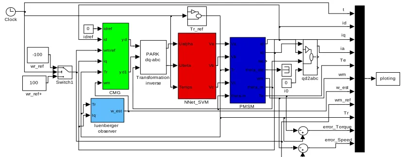
[image:2.612.99.513.149.311.2]The simulation method is designed with C Mex Files under Matlab/Simulink software.
Figure 1. Simulation Scheme Of Sensorless Sliding Mode Control Of A Permanent Magnet Synchronous Motor
2. DYNAMIC MODEL OF PMSM:
We admit that the machine is symmetric, that its induction has a sinusoidal distribution in the air-gap and that it is not subjected to the saturation. In the reference axis connected to the rotating field, the electromechanical behavior of the PMSM in the (dq) frame is expressed by the following equations [6]:
𝑈𝑑=𝑅𝑖𝑑− 𝜔𝑟𝜆𝑞+𝑑𝜆𝑑𝑡𝑑 (1)
𝑈𝑞 =𝑅𝑖𝑞− 𝜔𝑟𝜆𝑑+𝑑𝜆𝑑𝑡𝑞 (2)
𝜆𝑑=𝐿𝑑𝑖𝑑+𝜆𝑚 (3)
𝜆𝑞=𝐿𝑞𝑖𝑞 (4)
𝑇𝑒=32�𝜆𝑚𝑖𝑞+�𝐿𝑑− 𝐿𝑞�𝑖𝑑𝑖𝑞� (5)
𝑑𝜔𝑟 𝑑𝑡 = 𝑝 𝐽(𝑇𝑒− 𝑓𝑐𝜔𝑟− 𝑇𝑟) (6)
Where 𝑈𝑑 : Direct -axis stator voltage; 𝑈𝑞 : Quadrature -axis stator voltage; 𝑖𝑑 : Direct -axis stator current; iq : Quadrature- axis stator current; 𝐿𝑑 : Direct- axis stator inductance; 𝐿𝑞 : Quadrature- axis stator inductance; 𝜆𝑑 : Direct-axis stator flux; 𝜆𝑞 : Quadrature-axis stator flux; 𝑝 : Number of poles; 𝑅 : Stator resistance; 𝜆𝑚 : Rotor magnet flux linkage; 𝜔𝑟 : Mechanical rotor speed; 𝑓𝑐 : Coefficient of viscous friction; 𝑇𝑟 : Resistive torque; 3. PRINCIPLE OF VECTOR CONTROL: This technical consists to maintaining the reaction armature flux in quadrature with the rotor flux produced by the system of excitation like in case of the machine of DC. For an optimal working with a maximum torque, the simplest solution for a synchronous machine is to maintain the direct current equal to zero 𝑖𝑑= 0, and to control the speed by the quadrature current (𝑖𝑑) with the voltage 𝑈𝑞 [6][7][8]. By taking account of the equation (5) and by maintaining 𝑖𝑞 constant and𝑖𝑑= 0, the expression of the electromagnetic couple is written by: 𝑇𝑒=32𝑝𝜆𝑚𝑖𝑞(𝑡) (8)
By maintaining the conditions preceding, the equations of 𝑈𝑑 and 𝑈𝑞 are coupled, one is thus brought to establish a decoupling which consists the introduction of the compensation terms 𝐶𝑞 and𝐶𝑞. The tensions 𝑈𝑑 and 𝑈𝑞 depends respectively only by 𝑖𝑑 and 𝑖𝑞 (Fig 2). We are defining the compensation terms by: 𝐶𝑑=𝜔𝑟𝐿𝑞𝑖𝑞(𝑡) (9)
𝐶𝑞=−𝜔𝑟𝐿𝑑𝑖𝑞(𝑡) +𝜔𝑟𝜆𝑚
The fig.2 shows the decoupling of the system with the compensation terms.
t
id
iq
ia
T e
wm
w_est
wm_ref
T r
error_T orque
error_Speed 100
wr_ref+ -100
wr_ref
qd2abc
Tr
Iq w_est
luenberger observer 0
idref
ploting 0
i0 PARK
dq-abc
T ransformation inverse
T r_ref
Switch1
Va
Vb
Tr
Vc
theta-m id
iq
we
theta_ele
wm
theta_m
Te
PMSM Ualpha
Ubeta
Temps Va
Vb
Vc
NNet_SVM Clock
idref
id
wmref
iq
Tr
wm y d
y d1
Figure 2. Decoupling Of The System
4. SLIDING MODE CONTROLLER:
4.1 Principle of sliding mode controller:
The sliding mode control is to bring the trajectory state and to evolve it on the sliding surface with a certain dynamic to the equilibrium point. As a result the sliding mode control is based on three steps [10][17][11]:
4.1.1 Choice of the switching surface:
For a nonlinear system presented in the following form:
𝑋̇=𝑓(𝑋,𝑡) +𝑔(𝑋,𝑡)𝑈(𝑋,𝑡)
𝑋𝜖𝐼𝑅𝑛,𝑈𝜖𝐼𝑅𝑛,𝑟𝑎𝑛𝑔�𝑔(𝑋,𝑡)�=𝑚
Where 𝑓(𝑋,𝑡),𝑔(𝑋,𝑡) are two continuous nonlinear functions:
To determine the sliding surface, we take the form of general equation given by J.J.E.Slotine [10]:
𝑆(𝑋) =�𝑑𝑡𝑑+𝜆�𝑛−1𝑒(𝑋)
𝑒(𝑋) =𝑋𝑟𝑒𝑓− 𝑋
𝑒(𝑋) : denotes the error of the controlled greatness;
𝜆 : Positive coefficient;
𝑛 : Order of the system; 𝑋𝑟𝑒𝑓 : Reference greatness;
𝑋 : Variable of the controlled greatness. State;
4.1.2 The condition of convergence:
The condition of convergence is defined by the equation of Lyapunov [18], it make the surface attractive and invariant.
𝑆(𝑋)𝑆̇(𝑋)≤0 (12)
4.1.3 Control calculation:
The control algorithm is defined by the equation:
𝑈=𝑈𝑒𝑞+𝑈𝑛 (13)
With:
𝑈 : Control variable.;
𝑈𝑒𝑞 : Equivalent control variable;
𝑈𝑛 : Term of switch control variable. In order to reduce the chattering, the discontinuous function as exposed in equation (14) [20];
𝑈𝑛=𝐾𝑥𝑠𝑎𝑡�𝑆(𝑋)� (14) Where:
𝑠𝑎𝑡(𝑆(𝑋)∕ 𝛿) : function of saturation;
𝛿 : Width of the threshold of the saturation function;
𝐾𝑥 : Positive gain;
𝑠𝑎𝑡(𝑆(𝑋)⁄𝛿) =�𝑠𝑖𝑔𝑛�𝑆(𝑋)� 𝑖𝑓 |𝑆(𝑋)| >𝛿
𝑆(𝑋)⁄𝛿 𝑖𝑓 |𝑆(𝑋)| <𝛿
4.2 Strategy of regulation of PMSM on three surfaces:
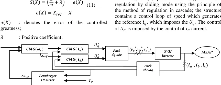
The figure (3) presents the diagram of the regulation by sliding mode using the principle of the method of regulation in cascade; the structure contains a control loop of speed which generates the reference𝑖𝑞, which imposes the𝑈𝑞. The control of 𝑈𝑑 is imposed by the control of 𝑖𝑑 current.
Figure 3. Schematic Global Of Sliding Mode Control With Strategy Of Three Surfaces
4.2.1 Control of speed:
The synthesis of control exploits the sliding modes technique, by using the principle of cascade adjustment method, which requires the choice of the surfaces that assure the objectives of control.
According to equations (5, 6), we notice that the relative degree of speed with 𝑖𝑞 is equal 1. So, in equation (11) we replace 𝑛 by 1, the surface selected for the control of speed error is:
𝑪𝑴𝑮(𝝎𝒓) 𝑪𝑴𝑮( 𝒊𝒒) Park
dq-abc
SVM Inverter
Leunberger Observer
𝑪𝑴𝑮( 𝒊𝒅)
MSAP
Park abc-dq 𝝎𝒆𝒔𝒕
𝑈𝑞∗
𝑈𝑑∗
(va*,vb*,vc*,) 𝒊𝒅𝒓𝒆𝒇
(𝒊𝒂 ,𝒊𝒃 ,𝒊𝒄)
𝑻𝒓 +
𝑅+𝐿𝑑𝑑𝑡𝑑
Id Vd1 Vd
-
Iq
Cd
-
+
𝑅+𝐿𝑞𝑑𝑡𝑑
Cq
Vq
Vq1
(10)
(11)
[image:3.612.89.521.479.646.2]ISSN: 1992-8645 www.jatit.org E-ISSN: 1817-3195
𝑆(𝜔𝑟) =𝜔𝑟𝑒𝑓− 𝜔𝑟 (16)
The derivative of the equation (16) is:
𝑆̇(𝜔𝑟) =𝜔̇𝑟𝑒𝑓− 𝜔̇𝑟 (17)
The law of control is defined by:
𝐼𝑞𝑟𝑒𝑓=𝐼𝑞𝑒𝑞+𝐼𝑞𝑛 (18)
We replace respectively the equation (5) in (6) and the obtained equation in (17), we obtain the following equation:
𝑆̇(𝜔𝑟) =𝜔̇𝑟𝑟𝑒𝑓−3𝑝2 �𝐿𝑑−𝐿𝑞𝐽�𝑖𝑑+𝜆𝑚𝑖𝑞+𝑇𝐽𝑟+ 𝑓𝑐
𝐽𝜔𝑟 (19)
If we replace the equation (18) in (19) we obtain:
𝑆̇(𝜔𝑟) =𝜔̇𝑟𝑟𝑒𝑓−3𝑝2 �𝐿𝑑−𝐿𝑞𝐽�𝑖𝑑+𝜆𝑚�𝑖𝑞𝑒𝑞+𝑖𝑞𝑛�+ 𝑇𝑟
𝐽 + 𝑓𝑐
𝐽𝜔𝑟 (20)
During the sliding mode we have:
𝑆(𝜔𝑟) = 0,𝑆̇(𝜔𝑟) = 0,𝑖𝑞𝑛= 0 (21)
We deduce the expression of 𝑖𝑞𝑒𝑞from (22):
𝑖𝑞𝑒𝑞=
𝜔̇𝑟𝑟𝑒𝑓+𝑓𝐽 𝜔𝑐 𝑟+𝑇𝐽𝑟
3𝑝
2 ��𝐿𝑑− 𝐿𝑞𝐽�𝑖𝑑+𝜆𝑚�
(22)
We replace equation (22) in (21) one obtains:
𝑆̇(𝜔𝑟) =−3𝑝2 ��𝐿𝑑−𝐿𝑞𝐽�𝑖𝑑+𝜆𝑚� 𝑖𝑞𝑛 (23)
During the mode of convergence, the derivative of the equation of Lyapunov must be negative:
𝑆(𝑋)𝑆̇(𝑋)≤0
According to the equation (15), the discontinuous function𝑖𝑞𝑛 defined by:
𝑖𝑞𝑛=𝐾𝜔𝑟.𝑠𝑎𝑡�𝑆(𝜔𝑟)� (24)
Kωr: Positive gain for speed regulator.
The control to the output controller of 𝑖𝑞𝑟𝑒𝑓 given by:
𝑖𝑞𝑟𝑒𝑓=
𝜔̇𝑟𝑟𝑒𝑓+𝑓𝐽 𝜔𝑐 𝑟+𝑇𝐽𝑟
3𝑝
2 ��𝐿𝑑− 𝐿𝑞𝐽�𝑖𝑑+𝜆𝑚�
+𝐾𝜔𝑟.𝑠𝑎𝑡�𝑆(𝜔𝑟)�
4.2.2 Control of id and iq currents: The expression of idis given by the equation:
d dtid=−
R Ldid+
Lq
Ldωriq+
1
LdUd (26)
We note that the equation (26), show the relative degree of current id with Ud is equal to 1. Therefore the error variable ed is given by:
𝑒𝑑= 𝑖𝑑𝑟𝑒𝑓 − 𝑖𝑑
The sliding surface of this control is given by:
S(id) = idref−id
The derivative of the equation of S(id) is:
𝑆̇(𝑖𝑑) =𝚤̇̇𝑑𝑟𝑒𝑓− 𝚤̇̇𝑑
If we replace the equation (26) in (27), the derivative of surface becomes:
𝑆̇(𝑖𝑑) =𝚤̇̇𝑑𝑟𝑒𝑓+𝐿𝑅 𝑑𝑖𝑑−
𝐿𝑞 𝐿𝑑𝜔𝑟𝑖𝑞−
1
𝐿𝑑𝑈𝑑 (28)
The low of control is defined by:
𝑈𝑑𝑟𝑒𝑓=𝑈𝑑𝑒𝑞+𝑈𝑑𝑛 (29)
During the sliding mode we have:
𝑆(𝑖𝑑) = 0,𝑆̇(𝑖𝑑) = 0,𝑖𝑑𝑛= 0
We deduce the expression of 𝑖𝑞𝑒𝑞from (30):
𝑈𝑑𝑒𝑞=�𝚤̇̇𝑑𝑟𝑒𝑓+𝐿𝑅 𝑑𝑖𝑑−
𝐿𝑞
𝐿𝑑𝜔𝑟𝑖𝑞� 𝐿𝑑 (30)
During the mode of convergence, the derivative of the equation of Lyapunov must be negative:
𝑆(𝑋)𝑆̇(𝑋)≤0
Consequently, the command to the output controller of 𝑖𝑑 becomes:
𝑈𝑑𝑟𝑒𝑓=�𝚤̇̇𝑑𝑟𝑒𝑓+𝐿𝑑𝑅𝑖𝑑−𝐿𝑑𝐿𝑞𝜔𝑟𝑖𝑞� 𝐿𝑑+𝐾𝑑𝑠𝑎𝑡�𝑆(𝑖𝑑)� (31)
𝐾𝑑R: Positive gain for 𝑖𝑑 current regulator.
In the same way to previous, by developing of the equation (32), the control to the output controller of 𝑖𝑞 given by (33):
𝑑 𝑑𝑡𝑖𝑞=−
𝑅 𝐿𝑞𝑖𝑞+
𝐿𝑑
𝐿𝑞𝜔𝑟𝑖𝑑−
𝜆𝑚
𝐿𝑞𝜔𝑟+
1
𝐿𝑞𝑈𝑞 (32)
𝑈𝑞𝑟𝑒𝑓=�𝚤̇̇𝑞𝑟𝑒𝑓+𝐿𝑅 𝑞𝑖𝑞−
𝐿𝑑
𝐿𝑞𝑝𝜔𝑟𝑖𝑑+ 𝑝𝜆𝑚
𝐿𝑞 𝜔𝑟� +𝐾𝑞𝑠𝑎𝑡 �𝑆�𝑖𝑞�� (33) 𝐾𝑞R: Positive gain for regulator of𝑖𝑞.
(27)
5. OBSERVER OF LUENBERGER
5.1. Principle of the observer
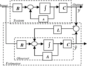
[image:5.612.311.524.99.335.2]The structure of an observer of state is illustrated by the figure (5), it is based on a model of the system, called the estimator or predictor, functioning in open loop. The complete structure of the observer includes a loop of corrective matrix gain, allowing correcting the error between the output of the system and that of the estimator [12] [13].
Figure 4. Structure Of An Observer Of State In Association With The System.
The dimensioning of corrective matrix gain L carried out to assure the convergence as soon as possible between the model of the estimator and the real system, Thus, by a wise choice of the matrix gain (L), we can modify the dynamics of the observer and consequently evolve the speed convergence of the error to zero, while preserving the condition on the matrix (A−LC) which must be a Hurwitz matrix [12], it means that its eigenvalues are with negative real parts in the continuous case, or have a module smaller than 1 in the discrete case.
5.2. Design of the observer of state:
The mathematical model of nonlinear states equations of PMSM is given by:
�𝑥̇=𝑦𝐴𝑥=𝐶𝑥+𝐵𝑢 (34)
With:
𝑢=𝑖𝑞 𝑥= [𝜃 𝜔 𝑇𝑟]
𝐴=�
0 1 0
0 −𝑓𝐽𝑐 −𝐽1
0 0 0
� (35)
𝐵=�0 𝑝𝜆𝐽𝑚 0�𝑇
The state equation of luenberger observer is given by [19]:
𝑑𝑥�
𝑑𝑡 =𝐴𝑥�+𝐵𝑢+𝐿(𝑥 − 𝑥�) (36) With:
𝐿=�𝑙0 0 02 𝑙1 0
𝑙3 0 0
� (37)
The observer state can be described by the following system [13]:
𝑑𝜃�𝑟
𝑑𝑡 =𝜔�𝑟
𝑑𝜔�𝑟 𝑑𝑡 =
1
𝐽 �𝑇𝑒− 𝑇�𝑟� − 𝑓𝑐
𝐽 𝜔�𝑟+𝑙1(𝜔𝑟− 𝜔�𝑟)
+𝑙2�𝜃𝑟− 𝜃�𝑟� (38)
𝑑𝑇�𝑟
𝑑𝑡 =𝑙3�𝜃𝑟− 𝜃�𝑟�
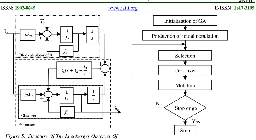
Figure 6 presents the functional diagram of luenberger observer. The estimated states are adjusted by the difference between the estimated �𝜃�� and the calculated (𝜃) position from equation of motor.
In matrix gain (37), the variable 𝑙2 determines the acceleration or the deceleration of the evolution of the variable estimated towards the real states. A greater gain will accelerate the process and a smaller gain will slow down it. The integral gains𝑙3 can reduce the static error to established regime of the observer [12].
The dynamics error of the observer is obtained from (34) and (36) by:
𝑒̇= (𝐴 − 𝐿)𝑒 (39) With:
𝑒=𝑥 − 𝑥� Observer
−
+
∫
A
B C
System
Estimator
L
∫
A
B C
Input Output
[image:5.612.98.283.226.371.2]ISSN: 1992-8645 www.jatit.org E-ISSN: 1817-3195
Figure 5. Structure Of The Luenberger Observer Of State.
The values of l1, l2 and l3 obtained by resolving the system (38) which based on mathematical equation of PMSM, are not exact and more suitable for PMSM drive. However we use genetic algorithm to optimize l1, l2 and l3.
6. NEURO SPACE VECTOR MODULATION
[image:6.612.90.524.68.305.2]The Neural network (NN) is the most generic form of Artificial Intelligence (AI) for emulating the human thinking process, is particularly suitable for solving many important problems as SVM. The NN uses a dense interconnection of computing nodes to approximate nonlinear function [14]. Using a general flowchart for neural network and the parameters presented in table 2.
Table 1. Nn Parameters
Parameters Value
Training Algorithm Backpropagation
Input layer 3 neurons
Hidden layer 15 tansig neuron
Output layer 3 purelin neuron
The neural network voltage selector is illustrated by figure 7.
Figure 6. Neural Network Voltage Selector
7. GENETIC ALGORITHM:
Figure 6 shows the flowchart of GA [15]-[16].
Figure 7. GA Flowchart
In order to the equation (45) with the system (19) a genetic algorithm is employed to optimize𝑙1, 𝑙2 and𝑙3 of control process. The configuration of genetic algorithm parameters used in this paper is given in Table 1.
Table 2. Ga Parameters
Parameters Value
Crossover probability 0,95
Mutation probability 0,001
Generation number Population 300
Population 200
Chromosome length 24 bit
The fitness function of each individual of this study is expressed by the equation (45):
𝑓𝑖𝑡𝑛𝑒𝑠𝑠=𝑀𝑂+ 21𝑆𝑇+ 1 (45) Where:
MO: represents the overshot. ST: represents the settling time.
8. RESULTS OF SIMULATION
5 parameters of PMSM:
The following table represents the parameters of PMSM:
Table 3. Parameters of PMSM
Parameter Value Unit
stator resistance. 1.4 Ω
d-axis inductance. 6.6 mH
q-axis inductance. 5.8 mH
magnetic flux constant 0.1546 Wb
Friction coefficient. 0.00038 N⋅m⋅rad−1⋅s−1
Motor inertia. 0.00176 Kg⋅m2
3 Vc
2 Vb
1 Va
In1 Out1
inverter
x{1} y {1}
Neural Network
emu
3 Time
2 Ubeta
1 Ualpha
Selection
Crossover
Mutation
Production of initial population Initialization of GA
Stop Stop or go No
Yes
+
+
−
+
−
Tr
Observer
Estimator
Iq 1
𝐽𝑠
fc
𝑝𝜆𝑚 1
𝑠
𝑙1𝐽𝑠+𝑙2−𝑙3𝑠
fc
𝑝𝜆𝑚 1
𝑠 1
𝐽𝑠
Bloc calculator of θr
+ −
−
[image:6.612.87.521.392.723.2]The matrix gains values of luenberger observer found by GA in this simulation is given by:
𝐿=�−9.70580𝑒+ 03 1.96230𝑒+ 04 00
7.2479𝑒+ 03 0 0�
6 SIMULATION RESULT:
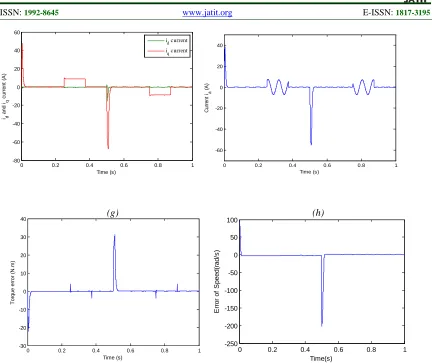
To illustrate the performances of the proposed method, we begin the simulation of PMSM without load, and at t= 0.5s we reverse the reference speed from +100 rad/s to − 100rad/s.
The load is applied in two periods:
𝜔𝑟𝑒𝑓=+100rad/s, the load (𝐶𝑟= 4𝑁𝑚) is applied at the moments 𝑡= 0.25𝑠 and it elimination at𝑡= 0.375𝑠.
𝜔𝑟𝑒𝑓=–100rad/s, the load (𝐶𝑟=−4𝑁𝑚) is applied at the moments 𝑡= 0.75𝑠 and it elimination at𝑡= 0.875𝑠.
The fig.9 shows, that the speed and torque response reach the references quickly with rejection of harmonic ripples (fig.9-a, b, c and d). In other hand the current 𝑖𝑑 is maintained null (𝑖𝑑= 0) and current 𝑖𝑞 is limited in an acceptable maximum value (Fig.9-e), and the statics errors, between the reference and actual Torque, and between the reference and actual speed are negligible (Fig.9-g and h).
0 0.2 0.4 0.6 0.8 1
-150 -100 -50 0 50 100 150
Time (s)
S
peed (
rad/
s
)
actual speed Estimated Speed Reference Speed
0.5 0.6 0.7 0.8 0.9 1
-110 -105 -100 -95 -90
Time (s)
S
peed (
rad/
s
)
actual speed Estimated Speed Reference Speed
0 0.2 0.4 0.6 0.8 1
-40 -30 -20 -10 0 10 20 30
Time (s)
T
or
que (
N
.m
)
Tem
Tref
0.245 0.25 0.255 0.26 0.265 0.27 0.275 0.28 0
1 2 3 4 5 6
Time (s)
T
or
que (
N
.m
)
Tem
Tref
(a) (b)
(c) (d)
ISSN: 1992-8645 www.jatit.org E-ISSN: 1817-3195
Figure 8. Simulated Speed (A), Zoom Of Speed (B), Torque (C), Zoom Of Torque (D), 𝑖𝑑 And 𝑖𝑞(E) Currents 𝑖𝑎(F), Torque Error (G) And Speed Error (H) Responses Of The PMSM Drive With Neuro Genetic Sensorless Sliding
Mode Control For A ±100 Speed Reference With A Fixed Charge Of ±4N.M
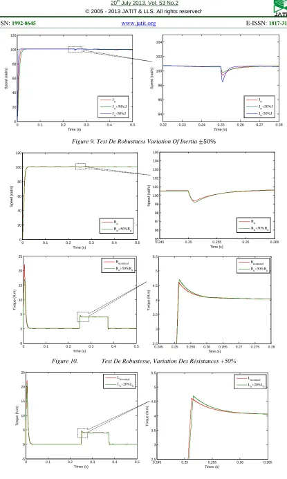
In order to test the robustness of the proposed control, we studied the influence of the variations parameters on the performances regulation of speed and torque.
Three cases are considered:
A variation of ± 50% on inertia, (Fig.9)
A variation of +50% on stator resistances, (Fig.10),
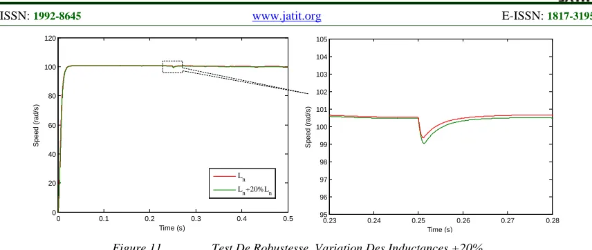
A variation of + 20% on stator inductances. (Fig.11)
To illustrate the performances of the control, we applied 𝐶𝑟= 4Nm load torque at 𝑡1 = 0.25𝑠 and we eliminate it at𝑡2= 0.375𝑠, with level speed reference +100 𝑟𝑎𝑑/𝑠.
0 0.2 0.4 0.6 0.8 1
-80 -60 -40 -20 0 20 40 60
Time (s) id
and i
q
c
u
rre
n
t (A
)
id current
iq current
0 0.2 0.4 0.6 0.8 1
-60 -40 -20 0 20 40
Time (s)
C
ur
rent
ia
(A
)
0 0.2 0.4 0.6 0.8 1
-30 -20 -10 0 10 20 30 40
Time (s)
T
or
que er
ror
(
N
.m
)
0 0.2 0.4 0.6 0.8 1
-250 -200 -150 -100 -50 0 50 100
Time(s)
E
rr
or
of
S
peed(
rad/
s
)
0 0.1 0.2 0.3 0.4 0.5
-5 0 5 10 15 20 25
Time (s)
T
or
que (
N
.m
)
Jn
Jn+50%J
Jn-50%J
0.24 0.25 0.26 0.27 0.28 0.29 0.3
2.5 3 3.5 4 4.5 5 5.5
Time (s)
T
or
que (
N
.m
)
Jn
Jn+50%J
Jn-50%J
Figure 9. Test De Robustness Variation Of Inertia ±50%
Figure 10. Test De Robustesse, Variation Des Résistances +50%
0 0.1 0.2 0.3 0.4 0.5
0 20 40 60 80 100 120
Time (s)
S
peed (
rad/
s
)
Jn
Jn+50%J
Jn-50%J
0.22 0.23 0.24 0.25 0.26 0.27 0.28
94 96 98 100 102 104
Time (s)
S
peed (
rad/
s
)
Jn
Jn+50%J
Jn-50%J
0 0.1 0.2 0.3 0.4 0.5
0 20 40 60 80 100 120
Time (s)
S
peed (
rad/
s
)
Rn
Rn+50%Rn
0.245 0.25 0.255 0.26 0.265
95 96 97 98 99 100 101 102 103 104 105
Time (s)
S
peed (
rad/
s
)
Rn
Rn+50%Rn
0 0.1 0.2 0.3 0.4 0.5
-5 0 5 10 15 20 25
Time (s)
T
or
que (
N
.m
)
Rnominal
R n+50%Rn
0.245 0.25 0.255 0.26 0.265 0.27 0.275 0.28 2.5
3 3.5 4 4.5 5 5.5
Time (s)
T
or
que (
N
.m
)
R nominal R
n+50%Rn
0 0.1 0.2 0.3 0.4 0.5
-5 0 5 10 15 20 25
Times (s)
T
or
que (
N
.m
)
L nominal Ln+20%Ln
0.245 0.25 0.255 0.26 0.265
2.5 3 3.5 4 4.5 5 5.5
Times (s)
T
or
que (
N
.m
)
ISSN: 1992-8645 www.jatit.org E-ISSN: 1817-3195
Figure 11. Test De Robustesse, Variation Des Inductances +20%
The simulation results presented in this part shows the robust of the Neuro-genetic sensorless VC with sliding mode controller of a permanent magnet synchronous motor using leunberger estimators, described in this papers, under stator resistance, moment of inertia and inductance variation. Figure 10 shows the stator resistance variation applied to examine our VC for PMSM drive by using novel estimator. In this case, the value of stator resistance was changed from the nominal value Rn to the +1.5Rn. Where, Figure 9 present the moment of inertia variation from Jn
to ±1.5Jn, and the inductance variation from Ln
to +1.2Ln, presented in Figure 11.
It’s seen in figure (9, 10 and 11) that the proposed speed controller allows to achieve a faster response and reject the harmonic ripples (motor parameters variations), as with nominal motor parameters. Also, a faster motor torque response has been achieved with proposed technique compared to the simulation with nominal case; as shown in figure (9, 10 and 11). Indeed, combining speed sliding controller and the novel estimator allow VC for PMSM to reject stator resistance, inertia and inductance variation due to this sliding controller, which is shown in figure (9, 10 and 11).
In conclusion simulations results are presented in figure 9; 10 and 11 show that the proposed controller is adaptive and robust to the effects of the variation of motor parameters such as stator resistance, stator inductance and moment of inertia on speed estimations, over a wide speed range, have been studied. Hence, the observer is more robust to parameter detuning.
9. CONCLUSION
In this paper, the results of simulation enabled us to judge qualities of the proposed control based on sliding mode variable structure controller. Through
the characteristics of the response obtained from simulation show that the control performances are very satisfactory. The dynamics of continuation is not affected during the variation of the load couple. The rejection of disturbance is very efficient. We notice, for speed, a fast starting with negligible overshoot and static error. The 𝑖𝑑 current is maintained null and independent of the torque. REFRENCES:
[1] Utkin V. I, “Sliding mode control design principles and applications to electrical drives,” IEEE Trans. on Industrial Electronics, vol. 40, No. 1, February 1993.
[2] S. Müller, “Doubly fed induction generator systems”, IEEE Industry Applications Magazine, vol. 8, n°3, pp. 26-33, May-June 2002.).
[3] T. Ming-Fa, T. Ying-Yu, “A transputer-based adaptive speed controller for AC induction motor drives with load torque estimation”.IEEE Transactions on Industry Applications, 1997, 33(2): 558-566.
[4] X. Dianguo, Y. Gao, “An approach to torque ripple compensation for high performance PMSM servo system”. PESC, 2004, vol. 5: 3256-3259.
[5] A. Qiu, B. Wu, H. Kojori, “Sensorless control of permanent magnet synchronous motor using extended kalman filter” Canadian Conference on Electrical and Computer Engineering, 2004, vol. 3: 1557-1562.)
[6] M.Ahmad “High Performance AC Drives: Modeling Analysis and Control”; Springer: New York, 2010.
[7] B. K. BOSE, “Power electronics and AC drives”, Prentice Hall, Englewood Cliffs, Newjersey, 1986.
0 0.1 0.2 0.3 0.4 0.5
0 20 40 60 80 100 120
Time (s)
S
peed (
rad/
s
)
Ln
L n+20%Ln
0.23 0.24 0.25 0.26 0.27 0.28
95 96 97 98 99 100 101 102 103 104 105
Time (s)
S
peed (
rad/
s
[8] Guy Sturtzer, Eddie Smigiel, “Modélisation et commande des moteurs triphasés”, Edition Ellipses, 2000.
[9] H De Battista and al. “Sliding mode control of wind energy systems with DOIG-power efficiency and torsional dynamics optimization”. IEEE Trans. Power Systems, vol. 15, n°2, pp. 728-734, May 2000.
[10] Slotine, J.J.E. Li, W., “Applied nonlinear control”, Prentice Hall, USA, 1998.
[11] Pierre Lopez and Ahmed Saïd Nouri, “Théorie élémentaire et pratique de la commande par les régimes glissants”, Collection: Mathématiques & Applications, Volume 55, springer, 2006). [12] George Ellis, “Observers in Control Systems, A
Practical Guide”, Academic Press, An imprint Elsevier Science (USA), Copyright 2002. [13] G. Zhu, L-A. Dessaint et al, “Speed Tracking
Control of the PMSM with state and load torque observer”, IEEE Trans. Ind. Electron, vol.47, No2, April, 2000, 346-355.
[14] Subrata K. Mondal, Member, IEEE, João O. P. Pinto, Student Member, IEEE, and Bimal K. Bose, Life Fellow, IEEE, “A Neural-Network-Based Space-Vector PWM Controller for a Three-Level Voltage-Fed Inverter Induction Motor Drive” IEEE transactions on industry applications, Vol. 38, No. 3, MAY/JUNE 2002, pp. 660-669
[15] A. El Janati El Idrissi, N. Zahid, “GA speed and dq currnets control of PMSM with vector control based space vector modulation using Matlab/Simulink®”, Journal of Theoretical and Applied Information Technology, 15st August 2011. Vol. 30 No.1.
[16] D.E Goldberg. “Genetic Algorithms in Search, Optimization and Machine Learning. ” Reading MA Addison Wesley, 1989.
[17] S-El-M.Ardjoun, M.Abid, A-G.Aissaoui, A.Naceri, “A robust fuzzy sliding mode control applied to the double fed induction machine”, International Journal Of Circuits, Systems And Signal Processing, Issue 4, volume 5, pp. 315-321, NAUN, USA, 2011.
[18] P.Lopez and A.S.Nouri, “Théorie Elémentaire Et Pratique De La Commande Par Les Régimes Glissants”, Springer, 2006.
[19] K. Nabti, K. Abed, H. Benalla “Sensorless direct torque control of Rushless Ac machine using Luenberger Observer”, Journal of Theoretical and Applied Information Technology, 31st August 2008 | Vol. 4 No. 8.