MULTIPLE MOBILE ANCHORS BASED LOCALIZATION
USING PARTICLE SWARM OPTIMIZATION (PSO) FOR
WIRELESS SENSOR NETWORKS
1S.KAVITHA, 2Dr.J.KANAKARAJ
1
Assistant Professor, Department of E.C.E, Hindusthan Institute of Technology, Coimbatore-641032. 2
Associate Professor, Department of E.E.E, P.S.G College of Technology, Coimbatore-641004. E-mail : [email protected]
ABSTRACT
In Wireless Sensor Network (WSN), though several works have been done on localization using mobile anchors, they cause huge delay in localization of the network since the mobile anchor has to cover the entire network. It will be difficult to provide maximum coverage to the entire network, without considering the visiting schedule of the mobile anchor node. In this paper, multiple mobile anchor based localization technique using Particle Swarm optimization (PSO) is proposed. PSO is used to determine the trajectory of the mobile anchor nodes which is based upon the node density and the distance between the nodes in the network. The mobile anchor nodes broadcast packets to the visited sensor nodes depending on the PSO visiting schedule. The non-localized nodes on receiving the packets, calculate the estimated distance between each of the mobile anchors and using trilateration method, they are localized. From the simulation results, it is proved that localization delay and energy consumption are reduced with increased packet delivery ratio, when compared to the existing approach.
Keywords: Wireless Sensor Network (WSN), Particle Swarm Optimization (PSO), Mobile Anchors,
Localization
1. INTRODUCTION
The continuous development in the field of communication networks has led to the emergence of a new technology, Wireless Sensor Networks (WSNs) for monitoring the physical world [1]. It is made up of some small sensor nodes which are distributed in an area and also collects information from their environments [2].The collection of this low-powered sensors dynamically form a network in the absence of any underlying infrastructure support [3].The sensors are used to sense the data from the environment, process the data, and to transmit the data to the base station directly or in multi-hop fashion [3].The sensing modality of each node is capable of communicating over wireless channel [1].Here each sensor could monitor only its region and the collected data is send to the sink node. The ability to correlate collected data in time and in space can be considered as the potential of WSNs [4].WSN can be deployed for a variety of tasks like detection, recognition, localization and tracking of objects or events of interest [5].It can be used in a wide range of application like battlefield surveillance, environment or health monitoring and disaster relief operations [5]
Localization is defined as the identification of the sensor node’s position in a sensor network. The accuracy of the localization technique is highly desired in any wireless sensor network [6]. The network includes a small number of anchor nodes. The position of these nodes is already known using GPS or are manually configured. The other nodes which don’t know their own position are called unknown nodes. Trilateral method can be used to figure the location when an unknown node knows three or more than three anchor nodes’ position information [7].Localization is a fundamental service as it is important to many applications like target tracking, intruder detection, environmental monitoring where the location information of the node is necessary. It is also relevant to many network main functions like routing, communication, cluster creation, network coverage, etc. [4].
sensors. Hence it becomes expensive for large networks. In range free technique, the anchor informs other sensors about its own position by message passing. Hence the complexity is reduced [8].Some of the aspects taken into consideration while designing or choosing a localization algorithm are limited resources, number and density of nodes, network topology, existence of obstacles or terrain irregularities, types of signal used and node mobility[4].
1.1 Need for Localization
Some of the advantages of localization are:
• Localization enables the efficient routing: In a sensor network, large number of nodes needs to communicate at a very short distance. The data collected by a node has to be sent to the central unit through several other nodes. Multi-hop routing is used to communicate the information. Hence it is necessary to have nodes of the same locality and to know their relative position with respect to their neighbors. Thus localization is very important.
• Localization provides the power saving: In the scenarios like pollution monitoring, the neighboring sensor nodes of the sensor network having same data which are not different from each other. Hence to save power the data from the neighboring nodes are combined .The combined and reduced data set is used for communication in order to conserve the power. The location information is necessary for the local data fusion. It shows the significance of localization.
• Localization assists in the applications like target tracking: In target tracking the range, speed and the direction of the target is needed to be determined. The sensors are deployed in region which sense the sign &from the moving target its range, direction, and speed can be monitored .hence the location of the sensor nodes is necessary to calculate the global orientation of the target.
• Localization useful in locating the source of the data: In event based sensor networks, the nodes are normally in sleep mode, the nodes awake only on the occurrence of an event. The data sensed and transmitted by the nodes requires a location stamp and hence localization is necessary [9].
1.2. Issues in Localization of WSNs
• The shortest path is used for unavailable distance measurements in centralizes localization algorithms such as the MDS
method. The shortest paths usually do not correlate well with their Euclidean distances in irregularly shaped sensor networks. Hence it leads to severe deterioration in the localization performance
• The GPS installation on each sensor node for location discovery is impractical due to its significant power consumption, cost and line-of-sight condition requirement. Also GPS receivers are susceptible to jamming and attenuations[10]
• The current generations of sensor nodes are smaller and cheaper. As a result the nodes have reduced memory and processing capacities and limited battery. In addition the nodes can only communicate with its local neighbors due to its short transmission range
• Some localization algorithm cannot be applied to low density WSNs as they cause considerable localization errors whereas the localization can be an expensive process using some algorithms in high density WSNs due to its high cost and high delay [4].
• Some of the localization algorithms the shortest path between a pair of nodes is calculated using the Euclidian distance. it is valid only if the shortest path is a straight line. This is not valid for network having concave topology as it gives distorted results. Some nodes gives good approximation whereas for others Euclidean distance differ significantly from the length of the shortest path.[4]
• The nodes positioned in the limits of the WSN area may not deal well localizing the nodes using some localization algorithm .hence the distance information each nodes can obtain is less and with lower quality.
• The proposed localization solution have low accuracy in obstructed environment as the existence of obstacles obstruct the line of -sight between the nodes. Signal reflection is caused by the obstacles and terrain irregularities which lead to wrong distance estimations. Both indoor and out door environments face this problem.
temperature has less effect on the signal whereas rain can affect the signal.
• If the node distribution is sparse or non uniform the performance and accuracy of Ad hoc Positioning System gets deteriorated greatly [3].
• Localization for large scale mobile underwater sensor networks is very challenging due to adverse aqueous environments, non-negligible node mobility and large network scale.
• Localization schemes designed for static sensor network runs periodically to update the location results. Hence the communication overhead increases dramatically.
• Distributed localization scheme designed for small scale underwater acoustics network is not suitable for large-scale underwater sensor network because of their slow convergence speed and high communication overhead [11].
• Localization has not been studied extensively in three dimensional WSNs because of its complexity [6].
1.3 Need for Solution
This paper tries to answer the following problems: How to reduce the delay involved in the
localization in case of single mobile anchor nodes.
How to determine the optimum visiting schedule of the mobile anchor nodes such that maximum coverage is obtained with reduced computational overhead.
How to reduce the energy consumption of sensor nodes involved in the localization process.
To solve the above problems, we propose a multiple mobile anchor based localization technique using Particle swarm optimization (PSO) technique for Wireless Sensor Networks (WSN). It consists of a set of three mobile anchor nodes for localization of the network.
Particle swarm optimization (PSO) is a popular multidimensional optimization technique. The strengths of PSO are ease of implementation, high quality of solutions, computational efficiency and speed of convergence [16]. PSO simulates the bird flock predatory behavior, each bird will be abstracted as a massless and sizeless particle to represent a candidate solution of the problem, the "particles" moves regularly and finds the optimal solution after a number of iterations in the solution space [17].
2. RELATED WORKS
Vibha Yadav et al [6] have discussed about a range free localization mechanism for WSN. It operates in a three dimensional space in this scheme. Here the sensor network is comprised of mobile and static sensor nodes. Mobile sensor nodes are equipped with GPS enabled devices so that their position at any instance can be known. The mobile nodes moving in the network space periodically broadcast beacon messages about their location. The messages are received by the Static sensor nodes as soon as they enter the communication range of any mobile node. The static nodes calculate their individual position on receiving the message based on the equation of sphere. When compared to existing approaches, the proposed scheme gains in terms of computational and memory overhead.
Hongyang Chen et al [8] have proposed a new cooperative localization scheme that can achieve high localization accuracy in mobility-assisted wireless sensor networks when obstacles exist. A convex localization algorithm has been presented to address the effects of non-ideal transmission of radio signals to consider the complex localization scenarios like the feasible set is empty. The localization accuracy is improved significantly even in the presence of mobile elements using the proposed cooperative localization scheme.
Hongyang Chen et al [12] have presented a new cooperative localization scheme that can achieve high localization accuracy in mobility-assisted wireless sensor networks in the presence of obstacles. A convex localization algorithm has been presented to consider the complex localization scenario, namely, the feasible set is empty. It addresses the effects of non-ideal transmission of radio signals. An optimal movement schedule for Mobile Elements (ME)s have been developed to achieve a shortest path under expected localization accuracy.
Jongjun Park et al [13] have proposed a localization method using mobile anchor trajectory. The mobile anchor broadcasts its locations periodically. The sensor nodes pair them with RSSIs and estimate the trajectory of the mobile anchor. The locations of the sensor nodes are calculated using two different trajectories. The sensor nodes do not use any additional H/W devices.
points. Each anchor point was equipped with the GPS. It moves in the sensing field, periodically broadcasting its current position. The sensor nodes compute their locations using the obtained the information. Here the sensor nodes do not need any extra hardware or data communication. Moreover, obstacles in the sensing fields can be tolerated.
Kezhong Liu and Ji Xiong [15] have presented a fine-grained localization algorithm for wireless sensor networks using a mobile beacon node. The algorithm uses RSSI for distance measurement. A GPS sender and RF (radio frequency) transmitter is attached to the beacon node and each stationary sensor node is equipped with a RF. The beacon node broadcasts its location information and stationary sensor nodes perceive their positions as beacon points. The location of the sensor node is computed by measuring the distance to the beacon point using RSSI.
From the literature review of existing works, we can say that, still there is need for multiple mobile anchor based localization scheme which answers all the problems listed in section 1.3.
3. MULTIPLE MOBILE ANCHORS BASED LOCALIZATION
3.1 Overview
The proposed technique uses PSO to determine the trajectory or visiting schedule of the three mobile anchor nodes based on the node density of the network.
Then based on the PSO based visiting schedule, when the three mobile anchor nodes traverse through the network, they broadcast packets which contain information regarding their id and location to the visited sensor nodes in the network. The unknown nodes having less received signal strength (RSS) value than the mobile anchor nodes on receiving the packet calculates the estimated distance between each of the mobile anchors to the unknown node. Each unknown node maintains anchor list having the anchor coordinates and estimated distance.
After that, Localization of the node is done using trilateration method. The unknown node will get two anchors from the list and localize them using trilateration method with the reference node. Reference node is the mobile anchor node having least distance to the unknown node.
The main advantage of the proposed solution is the usage of multiple mobile anchor nodes helps in reducing the delay due to the localization of the
network. Hence the localization of the network is carried out quickly. The PSO based approach for the visiting schedule of the mobile anchors enables it to traverse through the dense and sparse network with the same easiness. Hence the localization of both these networks is improved and the cost of localization is also reduced to a great extent.
3.2 Estimation of Node Density
A network consisting of several anchor nodes is considered and the local density is determined using the number of neighboring nodes. The node densities are classified into low, medium, and high. The ratio between expected hop distance and the transmission range for a particular local density is defined as the range ratio. The accuracy of the estimated hop-distance increases due to increase in number of categories at the cost of higher number of exchanged messages. Connectivity can be maintained using k number of neighbors in the wireless network.
Classification of density region depends on the number of neighbors. The region is identified as a low density region (L) when the number of neighbors is less than k. The region is identified as high density region (H) when the number of region reaches l. The region is considered as medium density neighbors (M) when the nodes are between k and l.
In the sensor network, reference nodes (RNs) contain a priori location information. The locations of other nodes are determined based upon the RNs.
In the sensor networks, when the hop-counts are propagated, the density awareness struggles to incorporate. Range ratio is represented as function of local density which is defined as the connectivity per unit transmission coverage. The RNs broadcast the hop-count and the nodes which hear the broadcast learn that they are one-hop neighbors of RN. Node’s local density determines the distance associated with each hop. The hop-distances at different node densities are gathered together using range ratio λ.
If a node within hearing distance from RN finds that it has high local density, it stores the range ratio, ∑λ1 = λH. On the other hand, if the node finds that it is located in medium or low density region, it
maintains
λ
λ
λ
λ
H Mor
∑
=∑
=1 1
respectively.
density to estimate range ratio and are gathered for forwarding. The received packets are discarded when the range ratio is higher than the existing value. When all the RNs broadcast their range ratio the process goes to an end.
If (n-1)th node is the previous node of (n)th node along a shortest multi-hop propagation path, then, the total range ratio accumulated by the (n)th node is
∑
∑
−= + =
= 1
1
, , ,
n
i i n L M H
n
λ
λ
whereλ
λ
orλ
λ
λ (1)The node has a higher probability of forwarding hop-count packets if the number of neighbors is higher. The nodes which are located at different directions and are close to transmission boundary receive the hop-count packet. The probability for the hop-distance to be closer to transmission range and at the direction that constitute shortest end-to-end path increases. The distance navigated becomes less than the transmission range when the number of neighbors is lower. The shortest end-to-end path is not provided for forwarding [18].
3.3 Estimation of Distance between Mobile Anchors
In this section, the Euclidian distance of one hop is estimated when an anchor node receives beacons from several other anchors. This is known as the correction factor. The equation (2) gives the correction factor handled by the anchor which is positioned at (xi,yi)
∑
∑ − + −
=
j j j
i
K y j yi x j xi CF
) ( )
( 2 2
(2)
Where K j is the number of hops between the current anchor, positioned at (xi, yi), and the anchor positioned at (xj, yj). The location of the sensor node can be estimated using the first correction factor. The consequent correction factors are disregarded. The sensor nodes which are in the neighborhood of the anchors provide the correction factor. The probability grid is quoted once the sensor node receives the correction factor. The hop-count to the set of neighbors, anchor node’s position, unit length of grid, and Euclidian distance estimate of one radio hop are the information contained in the sensor nodes at present.
Each node constructs the grid of arbitrary size which uses the position of at least three anchors and the unit length of the grid. The node density and the nodes in the network are specified for constructing
the grid of optimum size. Smaller grid sizes are adequate for higher densities of anchors in the network. The distances between the nodes are calculated as follows:
D = Distance between grid point and anchor / Correction factor (3) The computed D represents the distance, in hop count units, between the evaluated grid point and one anchor. [19]
3.4 Particle Swarm Optimization
Based upon the swarm intelligence, the particle swarm optimization (PSO) algorithm is proposed which solved the optimization problem in a search space. It also models and predicts the social behavior in the presence of objectives. It proves to be a stochastic, population-based computer algorithm which is based upon the swarm intelligence model.
The applications of swarm intelligence include social-psychological principles, approaches to social behavior and engineering applications. The fitness function is provided for evaluating the proposed solution. This communication structure or social network assigns neighbors for each individual for interaction.
The population of individuals is initialized and they are considered as random guesses at the problem solutions. These individuals are called the candidate solution or particles. In order to improve these candidate solutions, an iterative process is set. The fitness of the candidate solutions are evaluated by the particles and the information about the locations of best success are retained. This information is also available to their neighbors.
3.4.1 Estimation of Position and Velocity of the Particle
Each Particle in the swarm is represented by the following characteristics:
The current position of the particle
The current velocity of the particle
The population of the particles is used in the latest evolutionary optimization technique which is known as particle swarm optimization. In this algorithm, the particle corresponds to an individual and the position vector and velocity vector are updated by moving through the problem space.
) ( )
(
2 2 1
1 1
s rand
c s pbest rand
c V
V ki
k i i k
i k
i =w + × − + ×gbest−
+
(4)
V
s
s
ik+1= ki + ki+1 (5) Where,Vik is the velocity of i at iteration k,
s
ki is the current position of i at iteration k.c1 and c2 are positive constants and rand1 and rand2 are uniformly distributed random number in [0,1].
3.4.2 Optimization Function
Here the optimization function is calculated using the node density and the distance between the nodes.
∑
∑
+=
i B i D A f
λ η) . . 1
( (6)
Where λ represents range ratio and D is the distance between the nodes. A and B are the smoothing constants
The node density should be maximum and the distance should be minimum for the optimization function.
3.4.3 Weight Function
The inertia weight w weighting function in Eq (4), controls the momentum of the particle. The inertia weight can be dynamically varied by applying a scheme for the setting of the PSO, where w decreases over the whole run. The decrease depends on the start and end value of the weight given.
The Inertia term w, is provided with the below Eq (7) to make the convergence faster and easier.
β
* )
(
w
w
w
end start endw= + − (7)
where
) / ( 1
1 (
max
x
xα β
+
= )
wstart, Start value of the inertia weight wend, end value of the inertia weight x, current iteration number
xmax , maximum iteration number
α, used to manipulate the gradient of the decreasing factor
The inertia term should linearly decrease in order to facilitate exploitation over exploration in later states of the search.
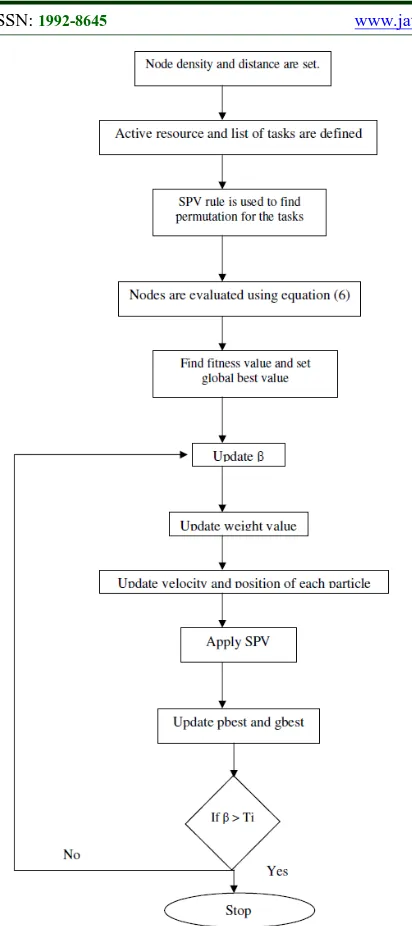
3.4.4 Visiting Schedule
Each particle represents a visiting scheduling scheme which uses n visiting schedules and m
number of anchor nodes.
x
ki is the position value ofith particle with respect to n dimension and
s
k i is
the sequence of tasks of ith particle in the processing order with respect to the n dimension.
The position vector
x
ikhas a continuous set of valuesThen the operation vector
r
ki is defined as,r
ki =s
ikmod m. (8) The Initial population of particles is constructed randomly for PSO algorithm. The initialized continuous position values and continuous velocities are generated by the formula,r
x
x
x
X
k0= min+( max− min)* (9)r
V
V
V
Figure 1: Flowchart For Scheduling
3.5 Localization using Triletaration
In this section, DV-hop algorithm is executed initially and the average distance per hop and anchor list for unknown nodes are accomplished. In DV-hop the position information is included in the packets which are generated by the anchor nodes. The numbers of hops away from the packets are denoted using a flag. In WSN, packets are broadcasted in the flooding mode. The hop number increases by one when they are transmitted by the relay nodes.
Using this hop number from a node to any anchor node can be determined. In the same way, the anchor nodes compute their hops to other
anchors also. The receiver estimates its distance to the anchor node when the information is sent to the unknown node. The location of the anchor node is determined only after getting three or more estimated values from the anchor nodes.
Then the anchors are chosen such that unknowns will get two anchors out of the list. Then the two nodes are combined with a reference node and are localized by trilateration. The unknown nodes receive average distance per hop initially from the reference node. During iteration, the reference node becomes unknown node, the unknown node becomes known node for which the coordinate is computed in the previous step. Trilateration gives N results which are compared with the actual coordinate. The coordinates which has the smallest difference after iteration, is saved. Ultimately unknown nodes also determine their positions.
Based on the PSO based visiting schedule, when the mobile anchor nodes traverse through the network, they broadcast packets which contain information regarding their id and location to the visited sensor nodes in the network. The unknown nodes having less received signal strength (RSS) value than the mobile anchor nodes on receiving the packet calculates the estimated distance between each of the mobile anchors to the unknown node. Each unknown node maintains anchor list having the anchor coordinates and estimated distance.
Figure 2: Trilateration
[image:7.612.318.521.460.665.2]Each node consists of an anchors list which records all other node’s coordinates and the estimated distances from them to U.
Node U randomly chooses two anchors from the other anchors and together with R to execute trilateration, records the result. Then we consider A7 as unknown node, and U as known node, and then execute trilateration again. Compare these results with A7’s actual coordinate, pick out the one which is the nearest to the actual value, and send it to U. Therefore, U will understand which result is the best, and it’s coordinate and the error will be recorded
Step 1: Initially the DV-hop algorithm is executed. The average distance per hop is computed and the unknown node save the value which they receive first and this is considered as the reference node. Each unknown nodes create an anchor list and the anchor’s coordinates are recorded. The distance from it to these anchors are also recorded.
Step 2: Any two anchors out of the list for each time is chosen and localized by trileration together with the reference node. Record the result. All the combinations should be included.
Step 3: Consider that D1 =4, D2 = 3, D3= 7, D4 = 6, D5 = 10, D6 = 9. Consider A7 as unknown node and U as known node, and displace A7 with corresponding Unknown node along with other two anchors to localize by trilateration.
Step 4: We will compare these coordinates’ error at R with the formula below. The true coordinate is (xr, yr), (x, y) is the estimate value in the computations:
% 100
)
(
)
(
2 2× +
+
−
−
y
x
y
y
x
x
r r
r
r
Let P1, P2,P3, P4, P5 and P6 be the estimated positions from the other anchors A1,A2,A3,A4,A5 and A6 along with U. Pick out the value which with the least error, assumed to be P2.
Step 5: A7 will send the estimated co-ordinate of U with respect to P2 , to the unknown node U.
Therefore, U will know P2 is the best result, and it will consider P2 as its coordinate.
Each unknown node will obtain their Positions. [7]
Since multiple mobile anchor nodes are used, it reduces the delay due to the localization of the network. Hence the localization of the network is
carried out quickly. The PSO based approach for the visiting schedule of the mobile anchors enables it to traverse through the dense and sparse network with the same easiness.
4. SIMULATION RESULTS
4.1 Simulation Parameters
We evaluate our Multiple Mobile Anchor based Localization using PSO (MMAL-PSO) technique through NS-2 [21] simulation. We use a bounded region of 500 x 500 sqm, in which we place nodes using a uniform distribution. The number of nodes is varied as 50,100,150 and 250. We assign the power levels of the nodes such that the transmission range of the nodes varies from 250 meters to 400meters. In our simulation, the channel capacity of mobile hosts is set to the same value: 2 Mbps. We use the distributed coordination function (DCF) of IEEE 802.11 for wireless LANs as the MAC layer protocol. The simulated traffic is Constant Bit Rate (CBR).
The following table summarizes the simulation parameters used
No. of Nodes 50,100,150 and 200.
Area Size 500 X 500
Mac 802.11
Simulation Time 20,30,40 and 50 sec
Traffic Source CBR
Packet Size 500
Transmit Power 0.660 w Receiving Power 0.395 w
Idle Power 0.035 w
Initial Energy 15.3 J Transmission
Range 250,300,350 and 400 m
Routing Protocol AODV
4.2 Performance Metrics
We compare the performance of our proposed MMALPSO method with the Mobile Anchor assisted node Localization (MAL) method [8]. We evaluate mainly the performance according to the following metrics:
Packet Delivery Ratio: It is the total number of packets received by the receiver during the transmission.
Average Energy Consumption: The average energy consumed by the nodes in receiving and sending the packets.
4.3 Results
A. Based on Nodes
In our initial experiment we vary the number of nodes as 50,100,150 and 200 with transmission range 250m and simulation time 50sec.
Nodes Vs Delivery Ratio
0 0.5 1 1.5
50 100 150 200
Nodes
D
el
iver
y R
at
io
MMALPSO
MAL
Figure 3: Nodes Vs Delivery Ratio
Nodes Vs Delay
0 1 2 3 4 5
50 100 150 200
Nodes
D
el
ay(
S
ec) MMALPSO
MAL
Figure 4: Nodes Vs Delay
Nodes Vs Energy
0 5 10 15 20
50 100 150 200
Nodes
E
n
er
g
y(
J)
MMALPSO
MAL
Figure 5: Nodes Vs Energy
Figure 3 show the Packet Delivery ratio occurred for both MMALPSO and MAL. As we can see from the figure, the delivery ratio is high for MMALPSO, when compared to MAL.
Figure 4 show the average end-to-end delay occurred for both MMALPSO and MAL. As we can see from the figure, the delay is less for MMALPSO, when compared to MAL.
Figure 5 show the Energy consumption for both MMALPSO and MAL. As we can see from the figure, the energy consumption is low for MMALPSO, when compared to MAL.
B. Based on Time
In our second experiment we vary the simulation time as 20, 30, 40 and 50 sec with 50 nodes.
Tim e Vs Delivery Ratio
0 0.2 0.4 0.6 0.8 1
20 30 40 50
Tim e(Sec)
D
el
iver
y R
at
io
MMALPSO
MAL
Figure 6: Time Vs Delivery Ratio
Tim e Vs Delay
0 2 4 6 8 10
20 30 40 50
Tim e(Sec)
D
el
ay(
S
ec)
MMALPSO
MAL
Figure 7: Time Vs Delay
Tim e Vs Energy
0 5 10 15 20 25
20 30 40 50
Tim e(Sec)
E
n
er
g
y(
J)
MMALPSO
MAL
Figure 8: Time Vs Energy
Figure 6 show the Packet Delivery ratio occurred for both MMALPSO and MAL. As we can see from the figure, the delivery ratio is high for MMALPSO, when compared to MAL.
Figure 7 show the average end-to-end delay occurred for both MMALPSO and MAL. As we can see from the figure, the delay is less for MMALPSO, when compared to MAL.
figure, the energy consumption is low for MMALPSO, when compared to MAL.
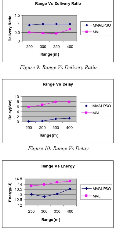
C. Based on Transmission Range
In our third experiment we vary the transmission range as 250,300,350 and 400m with 200 nodes.
Range Vs Delivery Ratio
0 0.5 1 1.5
250 300 350 400
Range(m )
D
el
iver
y R
at
io
MMALPSO
[image:10.612.99.289.180.553.2]MAL
Figure 9: Range Vs Delivery Ratio
Range Vs Delay
0 2 4 6 8 10
250 300 350 400
Range(m )
D
el
ay(
S
ec) MMALPSO
MAL
Figure 10: Range Vs Delay
Range Vs Energy
12 12.5 13 13.5 14 14.5
250 300 350 400
Range(m )
E
n
er
g
y(
J)
MMALPSO
MAL
Figure 11: Range Vs Energy
Figure 9 show the Packet Delivery ratio occurred for both MMALPSO and MAL. As we can see from the figure, the delivery ratio is high for MMALPSO, when compared to MAL.
Figure 10 show the average end-to-end delay occurred for both MMALPSO and MAL. As we can see from the figure, the delay is less for MMALPSO, when compared to MAL.
Figure 11 show the Energy consumption for both MMALPSO and MAL. As we can see from the figure, the energy consumption is low for MMALPSO, when compared to MAL.
5. CONCLUSION
In this paper, we have proposed a multiple mobile anchor based localization technique using Particle swarm optimization (PSO) technique. PSO is used to determine the trajectory of the mobile anchor nodes which is based upon the node density and the distance between the nodes in the network. We consider three anchor nodes for localization. The mobile anchor nodes broadcast packets according to the PSO visiting schedule. It contains id and location to the visited sensor nodes. The unknown nodes having less received signal strength (RSS) value than the mobile anchor nodes on receiving the packet calculates the estimated distance between each of the mobile anchors to the unknown node. Each unknown node maintains anchor list having the anchor coordinates and estimated distance. After that, localization of the node is done using trilateration method. The unknown node will get two anchors from the list and localize them using trilateration method with the reference node which is the mobile anchor node having least distance to the unknown node. From our simulation results, we have shown that the localization delay is reduced since multiple mobile anchor nodes are used and the visiting schedule of the mobile anchors enables it to traverse through the dense and sparse network.
REFERENCES
[1] Huang Lee and Hamid Aghajan, “Collaborative Self-Localization Techniques for Wireless Image Sensor Networks”, Conference Record of the Thirty-Ninth Asilomar Conference on Signals, Systems and Computers, 2005.
[2] Sadegh Zainalie, Mohammad Hossien
Yaghmaee, “CFL: A Clustering Algorithm For Localization in Wireless Sensor Networks”,
International Symposium on Telecommunications, pp.435-439, Dec 2008.
[3] Yun Wang, Xiaodong Wang, Demin Wang, and Dharma P. Agrawal, “Range-Free Localization Using Expected Hop Progress in Wireless Sensor Networks”, IEEE Transactions on Parallel and Distributed Systems, Vol. 20, No. 10, pp.1540-1552, Oct. 2009.
[4] Lina M. Pestana Leão de Brito, Laura M. Rodríguez Peralta, “An Analysis of Localization Problems and Solutions in Wireless Sensor Networks”, Polytechnical Studies Review, Vol 6, No.9, 2008.
Iterative Source Localization for Wireless Sensor Networks”, IEEE Transactions on Signal Processing, Vol. 58, No. 9, pp.4824-4835,Sept. 2010.
[6] Vibha Yadav, Manas Kumar Mishra, A.K. Sngh and M. M. Gore, “Localization Scheme For Three Dimensional Wireless Sensor Network Using GPS Enabled Mobile Sensor Nodes”, International Journal of Next-Generation Networks (IJNGN), Vol.1, No.1, Dec 2009. [7] Shuang Tian, Xinming Zhang, Xinguo Wang,
Peng Sun, Haiyang Zhang, “A Selective Anchor Node Localization Algorithm for Wireless Sensor Networks”, International Conference on Convergence Information Technology ,pp.358-362, 2007.
[8] Hongyang Chen, Qingjiang Shi, Pei Huang, H.Vincent Poor, and Kaoru Sezaki, “Mobile Anchor Assisted Node Localization for Wireless Sensor Networks”, IEEE 20th International Symposium on Personal, Indoor and Mobile Radio Communications, pp.87-91, 2009.
[9] Mayuresh M. Patil, Umesh Shaha, U. B. Desai, S. N. Merchant, “Localization in Wireless Sensor Networks using Three Masters”, IEEE International Conference on Personal Wireless Communications ,pp.384-388,2005.
[10]Yifeng Zhou and Louise Lamont, “An Optimal Local Map Registration Technique for Wireless Sensor Network Localization Problems”, 11th International Conference on Information Fusion, pp.144-151, sept.2008.
[11]Zhong Zhou, Jun-Hong Cui and Amvrossios Bagtzoglou, “Scalable Localization with Mobility Prediction for Underwater Sensor Networks”, The 27th Conference on Computer Communications INFOCOM. IEEE, pp. 2198 - 2206, April 2008.
[12]Hongyang Chen, Qingjiang Shi, Rui Tan, H.Vincent Poor, and Kaoru Sezaki, “Mobile Element Assisted Cooperative Localization for Wireless Sensor Networks with Obstacles”, IEEE Transactions on Wireless Communications, Vol. 9, No. 3, pp.956-963, March 2010.
[13]Jongjun Park, Seung-mok Yoo, and Cheol-Sig Pyo, “Localization using Mobile Anchor Trajectory in Wireless Sensor Networks”, International Conference On Indoor Positioning And Indoor Navigation, Sept. 2011. [14]Kuo-Feng Ssu, , Chia-Ho Ou, and Hewijin
Christine Jiau, “Localization With Mobile Anchor Points in Wireless Sensor Networks”,
IEEE Transactions on Vehicular Technology, Vol. 54, No. 3, pp.1187-1197, May 2005. [15]Kezhong Liu and Ji Xiong, “A Fine-grained
Localization Scheme Using A Mobile Beacon Node for Wireless Sensor Networks”, Journal of Information Processing Systems, Vol.6, No.2, pp-147-162, June 2010.
[16]Raghavendra V. Kulkarni, and Ganesh Kumar Venayagamoorthy, “Particle Swarm Optimization in Wireless Sensor Networks: A Brief Survey”, IEEE Transactions on Systems, Man and Cybernetics-Part C Application and Reviews.
[17]LIU Mei, HUANG Dao-ping, XU Xiao-ling, “Node Task Allocation based on PSO in WSN Multi-target Tracking”, Advances in Information Sciences and Service Sciences Vol. 2, No. 2, pp.13-18, Jun 2010.
[18]Sau Yee Wong, Joo Ghee Lim, SV Rao, and Winston KG Seah “Density-Aware Hop-Count Localization (DHL) is Wireless Sensor Networks with Variable Density” IEEE Communications Society / WCNC 2005.
[19]Radu Stoleru, and John A. Stankovic “Probability Grid: A Location Estimation Scheme for Wireless Sensor Networks” Sensor and Ad Hoc Communications and Networks, 2004. IEEE SECON 2004. 2004 First Annual IEEE Communications Society Conference. [20]Mr. P.Mathiyalagan, U.R.Dhepthie, and Dr.
S.N.Sivanandam “Grid Scheduling Using
Enhanced PSO Algorithm” (IJCSE)
International Journal on Computer Science and Engineering Vol. 02, No. 02, 2010, 140-145.
[21]Network Simulator: http//: