The nonlinear seismic response of tall shear wall structures

A thesis

submitted in partial fulfilment of the requirements for the Degree of

Doctor of Philosophy in Civil Engineering at the University of Canterbury

by

ROY GEORGE TAYLOR

University of Canterbury, Christchurch, New Zealand

motions.

ABSTRl\CT

New building codes are tending to place considerable value on of deterministic dynamic analyses as a means of assessing the of engineering structures to withstand severe seismic ground

An investigation of the more important factors affecting such an analysis, derived specifically for tall ductile shear walls, was undertaken. Initial considerations included the selection, and the derivation where necessary, of suitable structural idealisations, material constitutive relationships and numerical integration schemes, leading to an analysis which was sufficiently representative and

economically viable. The basic problem of program verification followed. Difficulties in ensuring that reliable accurate results were being obtained arose when certain types of structural idealisation and integration procedures were used. When these problems, which initially handicapped confident application of the program, had been satisfactorily resolved a sensitivity study of a realistic structure was pe rfo med . Results presented illustrate important characteristics of structural behaviour and the capabilities of the implemented analysis. Because it is vital that theoretical idealisations of reinforced concrete components should be based on experimental evidence, the case of slab coupling of shear walls was investigated with a sequence of reinforced concrete models. Interest was first concentrated on aspects of slab design, especially the control of punching shear within the range of deformations likely to occur in a seismic disturbance. Limited attempts were made to match standard idealised hysteretic relationships to the experimental responses to allow an improved dynamic analysis of structures incorporating these components. Finally, a pilot test of a slab

ACKNOWLEDGEMENTS

The research for this report was carried out in the Department of Civil Engineering, University of Canterbury, of which Professor H.J. Hopkins is Head.

Grateful acknowledgement is made of the support and guidance given to the candidate by the supervisors of his studies, Professor T. Paulay and Dr. A.J. Carr, by members of the staff of the

Department of Civil Engineering. and by fellow students.

Further assistance received from the following people is thankfully acknowledged:

Messrs. J. Sheard and G. Sims and the other technicians who worked on this project for their careful preparation of the test equipment and test specimens and for their assistance during testing.

Mr. H. Patterson for photographic work. Mrs. A. Watt for typing this manuscript. Mr. R. Powell for tracing many diagrams.

Mr. H. Watson for arranging for the purchase of materials and equipment.

The staff of the university's Computer Centre who made this project possible with their co-operation and friendly service.

ABSTRACT

ACKNOWLEDGEMENTS LIST OF FIGURES LIST OF TABLES LIST OF SYMBOLS CHAPTER ONE

CHAPTER CHAPTER 1.1 1.2 1.3 1.4 TWO 2.1 2.2 2.3 2.4 2.5 THREE 3.1 3.2 3.3 3.4 3.5 3.6 CONTEN'l'S

INTRODUCTION AND SCOPE OF RESEARCH Introduction

Philosophy of Dynamic Response Prediction The Dynamic Response Problem and the Scope of this Investigation

Format

COMPUTER PROGRAM RELIABILITY AND VERIFICATION Introduction

Verification Procedures Selection of Test structures Selection of Base Motions Extent of Verification

STRUCTURAL IDEALISATION OF A SLENDER SHEAR WALL Introduction

Fundamentals of Structural Behaviour

Assessment of Idealis.ations: A Utilisation of Previous Research

1 2 3 5 6 6 7 11 15 16 16 17 i i i x xv xvi

3.3.1 General 17

3.3.2 Elastic Analysis of Shear Wall Structures 17

3.3.3 Inelastic Analysis of Shear Wall 18

Structures

A Nonlinear Flexural Idealisation of Walls Finite Element Model A

3.5.1 General

3.5.2 Displacement Functions 3.5.3 Element Strains

3.5.4 Constitutive Relationships

3.5.5 Energy Solution for a Single Element 3.5.6 Force Computations

3.5.7 Evaluation of Element A stiffness ElementS: Simplified Integration

3.7

3.8 3.9

CHAPTER FOUR 4.1 4.2 4.3 4.4

4.5

CHAPTER FIVE 5.1 5.2 5.3 5.4 5.5 5.6

CHAPTER SIX 6.1 6.2

3.6.1 Description JU

3.6.2 Problems of Reduced Order Integration 31 Elements Cl and C2 : Lower Order Displacement

Functions

3.7.1 Description of Elements Cl and C2 3.7.2 stiffness of Elements Cl and C2 Further Elements

Transformations and Total stiffness Matrix Formation

SECTIONAL ANALYSIS Introduction

Assumptions and Limitations Nonlinear Section Theory

Component Constitutive Relationships 4.4.1 General Considerations

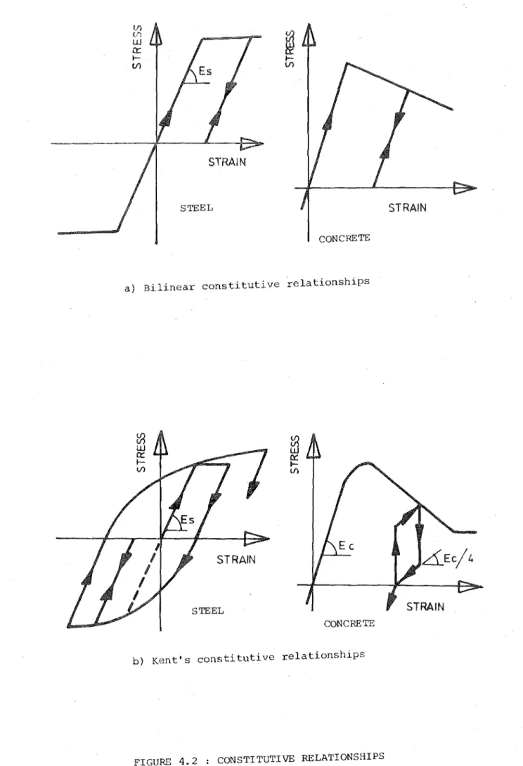
4.4.2 Selection of Constitutive Relations

32 32 32 33 33 36 36 36 39 39 39 4.4.3 Branch Points in Constitutive Relationships 40 4.4.4 possibilities in Future Refinements of

Constitutive Relationships 42

Discussion of the Implemented Analysis

INVESTIGATION OF NUMERICAL INTEGRATION TECHNIQUES Introduction

Implicit Integration of the Equations of Dynamic Equilibrium using Newmark's Constant Average Acceleration

(S =

Explicit Integration of the Equations of Motion 5.3.1 Selection of an Explicit Scheme for

Implementation

5.3.2 Mathematical Description

Methodology of Integration Scheme Evaluation Response Results

Choice of an Integration Scheme

IMPLICIT NUMERICAL INTEGRATION OF THE P.QUATlONS OF MOTION

Introduction

Integration Accuracy

6.2.1 Integration Accuracy Considerations in

6.3

6.4

CHAPTER SEVEN 7.1 7.2 7.3 7.4 7.S 7.6 7.7 7.8

6.2.2 An Illustrative Example

6.2.3 Equilibrium Correction 'l'ochniques 6.2.4 Out-of-phase Equilibrium Correction 6.2.5 Iteration on the Excess Force Vector 6.2.6 Total Equilibrium Iteration

6.2.7 Conclusions on Equilibrium Correction Techniques

6.2.8 Accuracy of the Representation of the Ground Motion Record

Integration Stability

6.3.1 Stability of Numerical Integration in Elastic and Inelastic Analyses 6.3.2 An Illustrative Example

6.3.3 Numerical Investigation

Convergence of the Numerical Integration 6.4.1 A Definition

6.4.2 An Illustrative Example

6.4.3 Bounding of the Convergence Limit THE COMPUTER PROGRAM STRUCTURE AND ITS APPLICATION

Introduction

Organisation of the Program 7.2.1 Summary

7.2.2 Reference Axis Locality 7.2.3 section Numbering

7.2.4 Organisation of Element Property Computation

7.2.5 Stiffness Matrix Changes

Member Ductility and Damage Assessment 7.3.1 Survival of the Structure

7.3.2 Secondary Damage

Damping and Mass Representation 7.4.1 Damping

7.4.2 Mass Representation

Data Files and Plotted Presentations Equation Solvers

Iteration and Equilibrium Correction Restart Capabilities

7.8.1 System Restart Capability

7.8.2 User Developed Restart Capability

Paqe

CHAPTER EIGHT 8.1 8.2

8.3

8.4 CHAPTER NINE

9.1 9.2 9.3 9.4 9.5 9.6 9.7 9.8 9.9

ELEMENT PERr'ORMANCE Introduction

Examination of Stiffness Matrices Depicting Nonlinear Behaviour

82

82

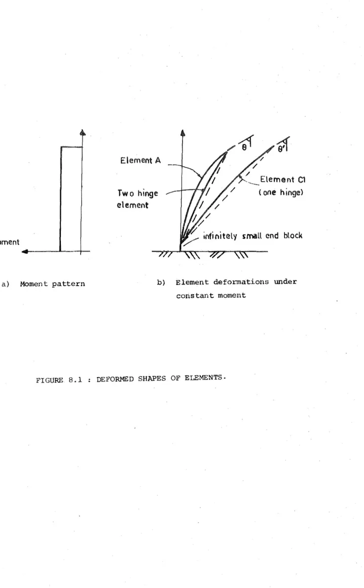
8.2.1 Illustrative Example 82

8.2.2 Deformations Under a Uniformly

Distributed Moment 83

8.2.3 Examination of Eigenvalues and

Eigenvectors of the Stiffness Matrices 83 Dynamic Analyses Using these Elements

8.3.1 Introduction 8.3.2 Element A 8.3.3 Element B

8.3.4 Elements C1 and C2 8.3.5 Two Hinge Element

8.3.6 Element A in a Realistic Environment Summary

STRUCTURAL RESPONSE STUDY Introduction

Scope of the Structural Response Study The Structure and its Des ign

Details of Structural Idealisation 9.4.1 Flexural Idealisation

9.4.2 Shear Modelling

9.4.3 Representation of Mass and Damping Selection of Earthquake Records

Summary of Santhakumar I s Analysis

Detailed Description of the Performance of the Basic Structure

9.7.1 General

9.7.2 Displacements

9. 7 .3 Behaviour of Coupling Beams 9.7.4 Wall Actions

9.7.5 Wall Stiffness Parameters 9.7.6 Moment CUrvature Relationships 9.7.7 Wall Shears

Response of the Basic Structure to a Ranqe of Base Motions

Progressive Modification of the Basic Structure 9.9.1 variation A

9.10

CHAPTER TEN

10.1 10.2 10.3 10.4

10.5

CHAPTER ELEVEN 11.1 11.2 11.3 11.4 ll.S 11.6

9.9.2 Variation B 9.9.3 Variation C 9.9.4 Variation D

Significant Observations of Behaviour and Design Recommendations

EXPERIMENTAL INVESTIGATION OF SLAB COUPLING OF SHEAR WALLS

Introduction

Summary of Previous Work

Objectives and Scope of this Investigation The Prototype Structure

10.4.1 Proportions of the Prototype 10.4.2 Design of the Prototype Slab Considerations for an Experimental Study

TEST SPECIMENS AND TEST PROCEDURES Introduction

Basic Test Configuration Model Limitations

Design of Test Structure Reinforcement 11. 4.1 General

11.4.2 Unit 1 11.4.3 unit 2 11.4.4 unit 3 11. 4. 5 unit 4 Instrumentation Page 123 125 125 130 132 132 133 134 134 137 137 139 139 142 143 143 145 145 147 147 150

11.5.1 General 150

11.5. 2 Force~Displacement Results 150

11.5.3 Displacement Profiles 150

11.5.4 strains in the Primary Seismic

slab Reinforcement 152

11.5.5 strains in the Special Transverse

Reinforcement 152

11.5.6 Beam Steel Strains in Unit 4 152 11. 5. 7 utilisation of a Structural Sceel Beam 156 11.5.8 Axial Elongation of the Coupling System 156

11.5.9 Stirrup strains 156

CHAPTER 'IWELVE 12.1 12.2 12.3 12.4 12.5 12.6 12.7 12.8 12.9 12.10 12.11

CHAPTER THIRTEEN 13.1

13.2

EXPERIMENTAL RESULTS Introduction

Strength and stiffness Degradation 12.2.1 Slab Tests

12.2.2 Unit 4

Deflection Profiles 12.3.1 Slab Tests 12.3.2 Unit 4

Stresses in the Longitudinal Seismic Reinforcement

12.4.1 Slab Tests 12.4.2 unit 4

strains in Secondary 010 Reinforcement Placed Transversely across Wall Toes Performance of the Structural Steel Beam 12.6.1 Unit 3

12.6.2 Unit 4

Beam Reinforcement strains in Unit 4 Elongation of the Coupling System Stirrup Behaviour

12.9.1 Slab Tests 12.9.2. Unit 4

Effective Slab Widths 12.10.1 Slab Coupling 12.10.2 Unit 4

Design Considerations

12.11.1 Interpretation of Results for the Design of Slab Coupling 12.11.2 Assessment of Beam-Slab

Interaction

A SUMMARY AND RECOMMENDATIONS FOR FUTURE RESEARCH

Dynamic Response study 13.1.1 Program Reliability 13.1.2 Mathematical Modelling 13 .1. 3 Numerical Integration 13.1. 4 structural Response Study

Experimental Study of Slab Coupling of Shear

Page 159 159 159 163 165 165 170 170 170 170 175 178 178 180 180 180 183 183 184 193 193 194 194 194 195 197 197 197 198 199

Walls 201

13.2.1 Slab Reinforcement Solutions and

REFERENCES APPENDIX A

A.I A.2 A.3 APPENDIX B

B.l

13.2

13.2.2 Composite Beam-Slab Action

EQUILIBRIUM CORRECTION PROCEDURES FOR SINGLE-DEGREE-OF-FREEDOM SYSTEMS

Out-of-Phase Equilibrium Correction Iteration on the Out-of-Balance Force

Iteration on the Total Equilibrium Equation EQUATION SOLVERS

Algol Equation Solver

Complementary Fortran Version

Page

203

A-I A-I

2.1 Structure A 9

2.2 Structure Al 10

2.3 structure B 12

2.4 Structure C 13

2.5 Impulse Functions 14

3.1 Element A 21

3.2 Incremental tangent and secant matrix definitions 21

3.3 Displacement definitions 26

3.4 Final simplified actions and deformations 26

3.5 Transformations 35

4.1 Description of the section 38

4.2 Constitutive relationships 41

4.3 Tangent stiffness determination during iteration 43

5.1 Simple model incorporating beam elongation modes 50 5.2 Comparison of explicit and implicit integration

schemes with an analytic solution 52

5.3 Undamped elastic response of the simple structure computed using the explicit scheme with different

time steps 52

6.1 Mode shapes and equilibrium correction forces for

Structure A 56

6.2 Out-of-phase equilibrium correction (1) 60 6.3 Out-of-phase equilibrium correction (2) 60 6.4 Comparison between iterative equilibrium correction

teChniques 63

6.5 Integration accuracy for elastic response to impulse

functions 63

6.6 Integration accuracy for inelastic response to impulse

functions 66

rl, '7 Intoqration accuracy for inelastic response to El Centro

N.S. ],940 ground motion 66

(j. fJ Spurious higher mode vibration in Structure A 70

b. lJ Accurate numerical integration where higher mode

t:eaponse is evident in structure A 70

b.10 Longer duration analyses with spurious vibration present 6.11 Effect of removing the higher natural mode on the

accuracy of integration

71

8.1 Element deformed shapes

B.2 Stiffness matrix eigenvalues and mode shapes

8.3 Displacement solution obtained using element A with 3 integration sections

8.4 Displacement solution obtained using element A with

5 integration sections

8.5 Displacement solutions obtained using element A with 7 integration sections

8.6 Displacement solution obtained using element B B.7 Identical displacement solutions obtained using

element Cl and the P.C.A. single spring hinge element 8.B Displacement solution obtained using element C2

8.9 Marginal stability when bilinear hinging is allowed at each end of the lower element

8.10 Satisfactory stability when hinging is allowed at each end of the lower element

8.11 Integration scheme accuracy for structure C Displacement solution comparison

8.12 Integration scheme accuracy for Structure C Moment solution comparison

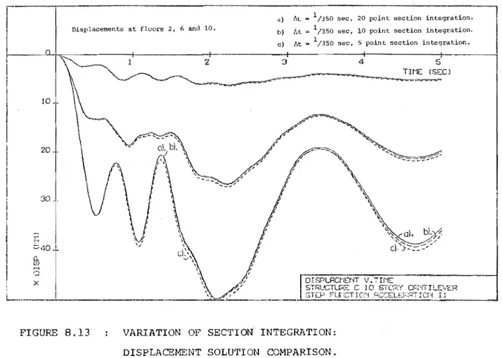
8.13 Variation of section integration: Displacement solution comparison

8.14 Variation of section integration: Moment solution comparison

8.15 Refinement of lower floor idealisation: Displacement solution comparison

8.16 Refinement of lower floor idealisation: Moment solution comparison

9.1 9.2 9.3 9.4 9.5 9.6 'L 7 9.9

The basic structure

Horizontal displacement history vertical displacement history

Axial force histories at each wall base Axial forces in the left-hand wall

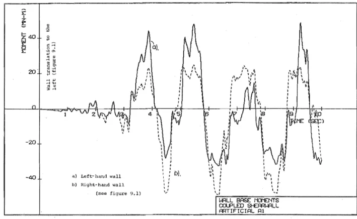
Wall moments on wall centreline at each wall base Momonts on the left-hand wall centreline

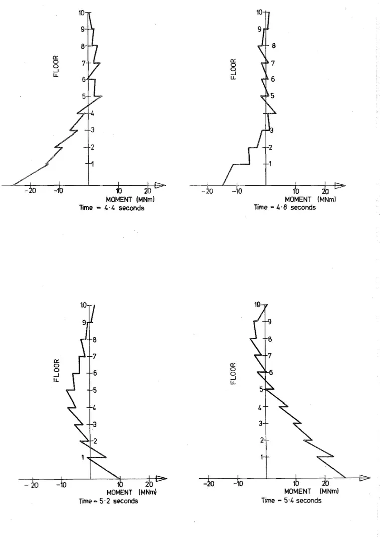
InBtrmtaneotls wall moment distributions

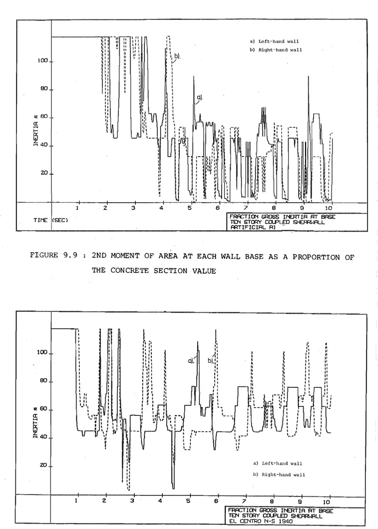
2nd mom~'nt of area at each wall base as a

prollortion of the concrete section value

9.10 lIistory of wall 2nd moment of areas for the El Centro response

9.11 Effective area at each wall base as a proportion of the gross concrete section area

9.12 Instantaneous stiffness centroid locality as a proportion of wall width

9.13 Moment curvature relationship in left-hand wall 115 9.14 Moment curvature relationship in right-hand wall 115 9.15 Moment curvature relationship at floor two in

the left-hand wall 116

9.16 Shear forces at wall bases 116

9.17 Wall shears in upper left-hand wall 118 9.18 Coupling beam moments and wall yielding in the

basic structure with the El Centre N-S 1940 excitation 118 9.19 Coupling beam moments and wall yielding in the basic

structure with artificial Al excitation

9.20 Coupling beam moments and wall yielding in the basic structure with artificial Bl excitation

9.21 Maximum displacements of the basic structure

9.22 Wall bending moment envelopes for the basic structure 9.23 Basic structure coupling beam rotations

9.24 Wall shear envelepes for the basic structure 9.25 Coupling beam moments and wall yielding in the

variation A structure with artificial Bl record 9.26 Coupling beam moments and wall yielding in the

variation B structure with artificial Bl record 9.27 Coupling beam moments and wall yielding in the

variation C structure with artificial Bl record 9.28 Coupling beam moments and wall yielding in the

variation D structure with artificial Bl record 9.29 Displacement envelopes for variations on the

basic structure

9.30 Wall shear envelopes for the modified structure 9.31 Coupling beam rotations for the modified structure

10.1 Plan of the prototype structure showing model locality

10.2 Elevation of the prototype showing model locality and a typical deformation pattern

11.1 Schematic illustration of test model 11. 2 '1'he test setup

11.3 Reinforcement in unit 1 11.4 Reinforcement in unit 2

11.5 Cage and structural steel for unit 3 11.6 Reinforcement for unit 4

11.7 Cross sections of units 1 - 4

11.8 positions of deflection measurements and assumed yield lines

11.10 pfender gauge positions on top and bottom reinforcement

placed transversely across wall toes 154

11.11 Unit 4 beam reinforcement and instrumentation 155 11.12 General view of the instrumentation 157

11.13 Loading sequence 158

12.1 Unit 1 force displacement response 160

12.2 Unit 2 force displacement response 161

12.3 Unit 3 force displacement response 162

12.4 Unit 4 force displacement response 164

12.5 Displacement profile of unit 1 at cycle 5 (~ = 3) 166 12.6 Displacement profile of unit 1 at cycle 17 (~ = 7) 166 12.7 Displacement profile of unit 2 at cycle 5 (~3) 167 12.8 Displacement profile of unit 2 at cycle 17 (~

=

12.10 Displacement profile of unit 3 at cycle 17 (~

=

168 168 170 170 12.13 Longitudinal seismic reinforcement stresses in unit 1 171 12.14 Longitudinal seismic reinforcement stresses in unit 2 172 12.15 Longitudinal seismic reinforcement stresses in unit 3 173 12.16 Longitudinal seismic reinforcement stresses in unit 4 174 12.17 Strains in unit 2 transverse reinforcement at wall toes 176 12.18 Strains in unit 3 transverse reinforcement at wall toes 177 12.19 Strains in the structural steel beam of unit 3 179 12.20 Strains in the structural steel beam of unit 4 181 12.21 Strains in the longitudinal beam reinforcement of unit 4 182

12.22 Strains in unit 4 beam stirrups 185

12.23 Unit 1 at ductility 3 186

12.24 Unit 1 at ductility 7 186

12.25 Unit 1 after disassembly 187

12.26 Partial failure of unit 1 187

12.27 unit 2 at ductility 5 188

12.28 Unit 2 at end of test 188

12.29 Unit 3 at ductility 3 189

12.30 Unit 3 at ductility 11 189

12.31 Unit 3 underside at ductility 11 190

Page

12.33 unit 4 at ductility 3 191

12.34 unit 4 at ductility 5 191

12.35 unit 4 at end of test 192

LIS T OF TABLES

7-1 Comparison of Computer Times

11-1 Test Setup Definitions for Use with Figure 11.2 II-II Main Features of the Slab Coupling Experimental

Investigation

II-III Material Properties

12-1 Coupling System Elongation

Page 79

141

LIST OF SYMBOLS

In the following list of symbols subscripts and/or superscripts have been left off some symbols. In these cases their use follows accepted patterns in signifying members of a series, the members of a vector or the elements of a matrix. Further definitions which relate to Appendix A are listed there.

Symbol b c b s e x f n q q

oq

..

c

variable thickness of concrete in section variable thickness of steel in section

eccentricity of stiffness centroid from reference axis spring stiffness

number of time steps nodal displacement

nodal displacement for linear increment arbitrary displacement

nodal displacement for transformed system time

displacement velocity acceleration base acceleration

transverse beam displacement used in element stiffness derivation

distance along length of beam element

distance from edge of section to stiffness centroid dimensionless distance (z

=

equivalent area of section

strain displacement relationship for element A

modified strain displacement relationship for element A modified strain displacement relationship for element A damping coefficient

tangent constitutive matrix secant constitutive matrix length of wall

Young's modulus of elasticity Voung's modulus of concrete

Young's modulus of elasticity relating to an equivalent section secant modulus

ET tangent modulus

Fe predicted force at the end of an increment which is consistent with the linearisation

Fr actually resisted forces computed from stresses Fxs excess force or out-of-balance force

H plastic hinge length

I moment of inertia

K stiffness

K tangent stiffness at beginning of increment o K K2 L M N N u N v P Q R Se Sr T. ~ T 9 U Z (: £ o

e

secant stiffness

7 x 7 stiffness for original element A simplified stiffness for element A

length of beam element mass

element A displacement function axial displacement function transverse displacement function

initially applied external static loads dynamic force of the Newmark

S ::;:

predicted element force consistent with a linearised increment

actually resisted element force at end of an increment transformation for i

=

combined transformation to global system potential energy

first moment of area of the equivalent section angle

factor applied to mass to represent damping Newmark's integration constant

factor applied to stiffness to represent damping denotes a relatively small quantity

angle of rotation of plastic hinge strain

strain at beginning of current increment angle

radius of curvature of equivalent plastic hinge length stress

concrete stress steel stress

Symbols

denotes an incremental part of the quantity it precedes

., .. denote the first and second deri vati ves with respect to time

CHAPTER ONE

INTRODUCTION AND OF RESEARCH

1.1 INTRODUCTION

Traditionally, rigid jointed frame structures have been accepted by engineers as most suitable for resisting seismic disturbances in a ductile manner. This was probably because their structural behaviour was more clearly understood and the analysis techniques were more fully developed for these than for other structural types.

More recently, interest in damage control, especially in the reduction of non-structural damage, has fostered increased interest in shear wall structures. One of the outstanding demonstrations of this was the performance of the Banco de America building, an 18-storey shear core structure, in comparison with a nearby similar size frame structure during the 1972 earthquake in Managua, Nicaragua [1,21. The comparatively light total repair cost and the rational seismic behaviour of the coupled shear wall structure has resulted in a more general acceptance of these structures as highly efficient and reliable lateral load resisting components.

In 1965 a long term research project examining shear wall structures was initiated at the University of Canterbury. The experimental

investigations consisted of a selective series of projects aimed at

examining, understanding and improving the performance of various components of shear walls. Studies related to conventional deep coupling beams [3J, diagonally reinforced deep coupling beams [3,4], shear strength of walls [5], diagonal cracking in tension walls [6], and construction joints in walls [7] have been undertaken. Numerous problems have been identified and improved solutions were suggested for the design of these individual components. In a major experimental program that followed the previous findings were combined to construct complete one-quarter scale structural models of seven-storey shear wall structures [8,9], the testing of which demonstrated tileir strength and ductility.

Significant progress has been made and is continuing with current similar tests [10]. However, at the end of any static testing program,

no matt~r how comprehensive, the following three unanswered questions will

i) What history of nonlinear deformation can be expected at critical locations during a major seismic disturbance?

ii) Which structural geometry, strength and stiffness

configurations will give optimum performance when subjected to particular types of earthquakes?

iii) What design criteria, including limit state analysis

procedures and detailing requirements, are necessary to ensure a design for a safe, reliable structure?

If a sufficiently refined and realistic structural idealisation for a time history dynamic analysis could be used i t should provide valuable information regarding the above problems.

A theoretical study of the nonlinear structural dynamics of frame structures has led to the development of a general purpose computer

program [12] which has provided a useful base on which to develop an analysis procedure for shear wall structures.

The research undertaken in this project has been directed towards answering the above three questions. It represents a continuation and merging of the two relevant fields of previous research, as outlined above.

1.2 PHILOSOPHY OF DYNAMIC RESPONSE PREDICTION

The analysis of structural systems subjected to seismic loading may be said to be an empirical science; one based upon observation and experiment. As such, it is supposed to be verifiable, that is, capable of calculating beforehand results subsequently confirmed by observation and experiment. In fact it is only partially verifiable. That is to

H~y, a certain displacement history will exist if a certain building,

POIHw:-wing certain mass, stiffness and damping characteristics, is Hubjocted to a particular ground motion. In order to make absolute prodictions of response, deterministic rather than probabilistic information relating the relevant structural variables is required.

In assessing the response results presented in this thesis

scientific caution must be applied. It is important to avoid confusion botwO€ltl what is inferred and what is in fact determined. Although

derived from a probabilistic assessment of a large body of results, should be accf.lpted as reliable.

The role of approximate, but practical, analyses in understanding structural behaviour is a vital one. The importance of knowledge gained by mathematical model prediction is that it.enables us to progress beyond the limits of our present experience. In view of the narrow range of our immediate experience (derived from model tests and actual seismic events) these analytical results are vital, but until the phenomena involved are more fully understood much of our knowledge must remain approximate.

1.3 THE DYNAMIC RESPONSE PROBLEM AND THE SCOPE OF THIS INVESTIGATION It appears that three distinct problems, belonging to different studies and requiring different methods for their solution, require attention in any effort to predict nonlinear structural responses. There is a problem of determining an appropriate base acceleration

function, a problem of selecting a representative structural idealisation and a problem of establishing a reliable piecewise numerical integration technique. Of these three, the base acceleration problem remains poorly defined and difficult to deal with; the numerical integration problem is partially solved in that reliable techniques are now available; the problem of structural idealisation, particularly the representation of shear walls, has often been oversimplified and consequently many models are of limited applicability.

In the above context the scope of this work is briefly outlined as follows:

a) Base acceleration

The selection of an earthquake record for a deterministic anltlysiR i.s a highly subjective process and although about 15 strong motion historical records are available at the present time, ground motion intensity and characteristics for a particular shock vary widely with distance from the epicentre and differing geological conditions. Mor<wver, repeatability at a particular site cannot be assured so that an historical record may not be representative of a future event. Further brief reference is made to earthquake record selection in Chapter 9 where

b) Numerical integration

Newmark's constant average acceleration scheme [11] has been shown by many investigators to provide accurate, economical solutions for a wide range of problems. Most studies on numerical integration, however, examine elastic structures to gauge the techniques. In fact, it is

probable that the effects of a variable structural stiffness upon the accuracy and stability of the integration scheme will be significant. Adaption and implementation of iterative and out-of-phase equilibrium correction procedures, to accommodate the highly interactive nonlinear effects, proved to be important developments in the integration of non-linear problems.

It has been suggested [12] that an explicit numerical integration scheme may provide a more efficient means of solution to continuously variable nonlinear problems than implicit integration schemes (see Chapter 5) which require numerous stiffness matrix operations. An exploratory study was performed to gauge the usefulness of explicit

integration compared with implicit methods for the analysis of shear walls.

c) structural idealisation

A range of structural models varying in detail of modelling and complexity may be considered. There are the simple and efficient pure elastic beam and lamina models which lead to economical solutions which have been extensively used in the past [13]. An elastic

approximation, however, cannot always provide reliable results in a

dynamic analysis. Nonlinear static analyses using refined isoparametric finite element models, with superimposed concrete and steel elements, have also been performed [14]. This extremely detailed modelling is

considered to represent the forefront of present feasibility for nonlinear static analyses but is, because of the-qomputational effort required, boyond the limits of practicability for a full scale dynamic analysis. Howover, it should be possible to find, somewhere between these extremes,· a practical model which is sufficiently realistic in its idealisation of shear walls.

A major part of the research effort reported here was absorbed in identifying suitable elements, implementing them in a dynamic analysis program, and examining their merits. It must be recognised that any mathematical model, based on approximating assumptions, cannot be proved

phenomena of the prototype, can provide verification. one example of such an experimental model investigation was undertaken here where the slab coupling of shear walls was considered.

1.4 FORMAT

chapters 2 - 9 of this thesis present theoretical studies in which a refined analysis, intended for the dynamic analysis of shear walls, is discussed while in Chapters 10 12 the experimental investigation of shear wall coupling systems is described together with attempts to calibrate simplified mathematical models. A summary and suggestions for future

CHAPTER TWO

COMPUTER PROGRAM RELIABILITY AND VERIFICATION

2.1 INTRODUCTION

with the development of larger and more complex dynamic analysis computer programs, the problem of program verification [81] becomes

increasingly more difficult. Even though a program is based on generally accepted theory it cannot be verified with just normal use and a review of the printout. Certainly any major errors will be detected with use of the program, but any perturbation which does not disturb the response results beyond the threshold of obvious error may not be detected by the user.

There are two relative situations which are widely recognised in program verification: One where the program has been written in-house and the programmer is in qirect contact with all program use; the other where the program has been obtained externally and the users, typically, have only limited knowledge of the program structure and often do not fully appreciate any limitations of the mathematical models. The first situation is the one applicable to this development and it is, clearly, the most reliable, particularly when different structural types and newly developed models are considered. The second situation in the case of any nonlinear structural dynamics program must, with the knowledge available at present, be of limited reliability. The basic problems exposed by Sharpe [12] and the inherent but undefined approximations in recently published shear wall response studies [15,16], attest to this fact. This second situation is, unfortunately, the one in which most designers are likely to be placed when attempting nonlinear dynamic analyses.

2.2 VERIFICATION PROCEDURES

Many verification procedures, particularly those applied to programs written for theses, are haphazard processes at their best. The program is

usually written to solve a problem of particular interest, but it may be computationally possible to apply the program to a wide range of problems. Meanwhile, it is probable that the program was verified only for the

be applicable to the original problem. Oversight of this second simple but fundamental principle would appear to be particularly prevalent in the application of nonlinear frame analyses to shear wall structures.

In an effort to ensure a high level of verification the following general procedures were involved:

i) Independent subroutine strings were used to compute the stiffness of different element types.

ii) stiffness parameters were monitored to ensure that each element was functioning correctly as nonlinear excursions occurred.

iii) Cross checking was achieved by re-analysing a structure with five different elements available in the program.

iv) Convergence studies were carried out with refinement of the idea lisa tion .

v) Convergence studies with time step reduction to examine the equilibrium correction techniques and overall integration accuracy were performed.

vi) Three different, completely independent programs were used to compare damped elastic responses computed by analytic

and implicit integration methods.

explicit integration

vii) Comparisons between analyses were made by matching accurately plotted graphs rather than by comparing point values. Many of the actual comparisons on which important conclusions are based are presented in this report.

More specific consideration in achieving these checks is given in the next section.

2.3 SELECTION OF TEST STRUCTURES

Program verification, idealisation accuracy and integration stability ilElSeSsment are, by their nature, difficult when the proposed dynamic

cmalysis (see Chapter 3) is undertaken. Only a carefully planned, mllLhodicill progression from simple verifiable exampl'es to large scale analyues can produce a reliable program.

'I'le procedure adopted commences with a highly simplified structure, used as iJ debugging tool, verifying the basic operation of the program. This was

tht~ simple elastic portal frame structure, used in Chapter 5 to confirm

increasingly more complex structures were then used to examine varioLls aspects of the integration process. 1\s the structures became more complox, interpretation became more difficult and monitoring of parameters bL'came more expensive.

Three further basic test structures (figures 2.1 to 2.4) were derived and analysed repetitively. Of these three, structure 1\ was intended primarily for the numerical integration investigation and a single simple bilinear element was used exclusively; structure B, a modification of structure 1\, was derived specifically to allow comparison between the different

idealisations, although a limited integration accuracy study was also performed; structure C was designed as a realistic example to investigate accuracy and stability criteria in the total analysis context.

1\ more detailed description of these structures is given as follows: (a) structure A

This structure (figure 2.1) comprises a single elasto-plastic element representing a cantilever with all yield occurring at the base. The following structural attributes represent an attempt to achieve

simplicity of the response and confirmation of the numerical integration: i) A single element structure was chosen for simplicity in result interpretation.

ii) Yield levels and stiffness values were selected so as to ensure a vigorous response in the nonlinear range.

iii) The longest natural period of the structure was shorter than is typical for tall shear wall structures.

iv) A short period mode was included to identify its role in the response.

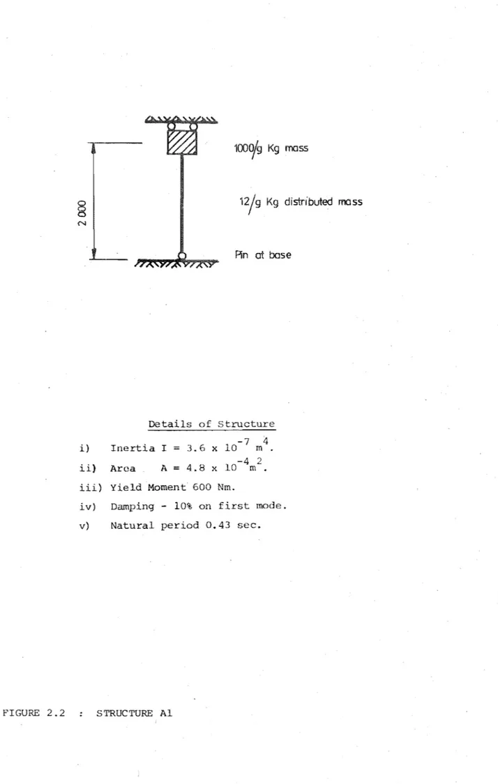
v) Modification of the basic structure A was made to obtain structure Al (figure 2.2) which possesses an identical first mode period wi th the higher transla tiona1 mode suppressed.

(b) structure B

This structure (figure 2.3) is similar to structure A with plastic hinging allowed only in the lower element and it retains most of

1000/g Kg mass

12/9 Kg distnblted mass

Details of Structure

i) Inertia I 3.6 x 10- 7 m 4 ii) Area A ₌₌ 4.8 x 10-4 m 2

.

iv) Damping - 10% of critical on first two modes.

v)

FIGUHE 2.1

Natural periods of two translational modes: 0.43 sec., 0.0062 seC.

§

N

i) Inertia I ii) Area A

12/9 Kg distributed mass

An at base

of structure

3.6 x 10-7 m4.

-4 2

4.8 x 10 m. iii) Yield Moment 600 Nm.

iv) Damping - 10% on first mode. v) Natural period 0.43 sec,

ii) Additional short period modes were incOrpOr[ltod and tllt'"p could be controlled, to some extent, by nodal mass assignment.

(c) Structure C

Finally, a ten-storey reinforced concrete cantilever was examined (figure 2.4). This structure, considered to be representative of a typical shear wall, was proportioned to make definite demands on the numerical technique in areas where weakness had previously been encountered. It has the following outstanding characteristics:

i) Only elements of the lower two floors allowed nonlinear behaviour. This resulted in a structure which was easily analysed and

that provided an acceptable environment in which to test selected elements. ii) Equal steel areas in each face of the wall were provided.

In the absence of dead lead this can result in large and sudden changes in axial stiffness. Therefore, the model allows stringent testing of equilibrium correction techniques.

iii) The selected relatively long first mode period, together with a short period base motion, causes a series of nonlinear waves to propagate up the structure.

Although this structure has a long first natural period

(2.46 seconds) consideration of alternative versions, with reduced masses and longest natural periods of 1.61 and 1.12 seconds, revealed the original structure to make the most severe demands on equilibrium correction

techniques.

2.4 SELECTION OF BASE MOTIONS

For the most part, while testing the above three structures, the simple arbitrary ground motions II and I2, shown in figure 2.5, were used. They proved ideally suited to this portion of the investigation for the

following reasons:

i) The .cyclic but simple functions give an easily assessable response.

ii) A vigorous initial excitation of the structure into the nonlinear range required considerable equilibrium correction.

iii) Zero excitation is present during the final portion of the rOf;ponse so that, as inertial and damping forces diminished, a simple ('qui libri.um check became available.

i)

8

o

N

ii) o o

(0

8

..

N

Details of

-Inertia I Area A " .

Structure 3.6 x 10- 7 4.8 X 10- 4

iii) Yield Moment 600 N-m.

12/9 Kg distributed mass

Lower node is assigted a portion cJ dIStributed mass

4 m

2 m

.

iv) Damping - 10% of critical on first two modes.

v} Natural periods of translational modes -0.43 t 0.098 t

0.0067 I 0.032 sec.

r

1

0

0

0

§

0

~

0

SE k:tion@

®

®

®

9th

8th

- 7th

1 - 6th

5th

!-4th

-.3rd

-2nd

-1st

(b) Section

®

(e) Section

®

(d) Section

®

lovver two floors only)

77,·, ",,,

al

FIGURE 2.4

structure

i) Steel Properties: Yield stress Young's Modulus E ii) Concrete properties:

280 MPa 200,000 MPa.

Crushing strength f' = 21 MPa Modular Ratio

g

natural modes.

v) Periods of first two natural modes: 2.46 sec., 0.42 sec.

TIME (sec.)

-0·39

oj IMPULSE ACCELERATION FUNCT10N 11

se cond offset 0·3g-l--__

-0·39 TIME (sec)

b) IMPULSE ACCELERATION FUNCTION J 2

v) Acceleration functions II and I2 were also found to be

slightly more difficult to integrate with structure A and considerably more difficult with structure C than was the El Centro 1940 N-S ground motion. Thus conclusions drawn from the use of the acceleration functions II and 12 and applied to the integration of recorded ground motions should be conservative in most cases.

2.5 EXTENT OF

Considerable efforts have been made to ensure that, using the program developed, reliable results could be obtained for any shear wall for which a flexural model is appropriate. The actual verification process is spread throughout the following six chapters of this thesis and is related to particular developments as they are discussed. The structures and acceleration functions described represent a small portion of the test runs actually performed, but they are considered to be

sufficient to illustrate the. approach taken in this study, some of the major problems encountered and, of course, to confirm any conclusions drawn. However, the program must still be strictly classified as a research tool and although it is based upon sound, versatile theory being highly suitable for future development, it is without the benefit of widespread application. Prospective users are warned that this, and other developmental nonlinear dynamic analysis programs, should be used with caution, preferably with understanding of the theory involved and with some knowledge of the program structure.

assessment of any results is essential.

CHAPTER THREE

STRUCTURAL IDEALISATION OF A SLENDER SHEAR WALL

3.1 INTRODUCTION

The realistic determination of the response of reinforced concrete structures requires knowledge of the inelastic behaviour of the component materials, as well as the ability to incorporate this information into a rational analysis of real structures. Inevitably, an acceptable

compromise between reality and computational simplicity is required. While numerous successful nonlinear dynamic analyses have been

performed with different structures, only a small portion of the literature on shear walls describes dynamic response determination. This is

particularly true of nonlinear responses [I, 15, 16, 17] and in only one of these [15] is the structural model thoroughly described. Meanwhile, a considerable number of nonlinear static analyses, applicable to shear walls, have been performed, in some cases to quite high degrees of refinement [18,19,20,21,22,23,24,25].

The particular structural type of interest is the slender shear

wall, defined in the following section, for which the selected elements have been specifically derived. Consideration has been given to a

variety of idealisations, together with previous experimental and analytic work, to select a group of elements for further detailed investigations

to achieve an improved idealisation of the structure [26,27].

3.2 FUNDAMENTALS OF STRUCTURAL BEHAVIOUR

For the purposes of this study the slender shear wall may be a single cantilever or it may consist of two or more coupled walls which in each case should have a height to length ratio of 3 or more so that flexural theory is directly applicable. Only those structures exhibiting a ductile moment failure mechanism, where shear, bond slip and other types of brittle failure are suppressed, are readily amenable to the proposed inelastic analysis.

'!'he following distinctive features of the structural type are significant when a dynamic response investigation is contemplated:

i) Each wall tends to deform as a single cantilever exhibiting overall simplicity of structural action.

iii) Substantial shear forces of alternating sense, transmitted from coupling beams, will have large and diverse effects on the moment-curvature relationships of complex wall sections.

iv) For elastic beam element solutions, very large wall lengths relative to the corridor width do not invalidate the assumptions of model application. It is possible, however, that large wall lengths combined with nonlinear behaviour may do so.

v) Rotational inertia associated with walls will be greater than for frames.

vi) Stress concentrations at the junction of walls and coupling beams may require consideration.

vii) Shear deformation due to sliding shear and diagonal cracking is likely to be significant in certain cases.

In the search for a suitable idealisation, attempts have been made to recognise these distinctive features, taking advantage of them where possible and incorporating capabilities in the model where necessary.

3.3 ASSESSMENT OF IDEALISATIONS A UTILISATION OF PREVIOUS RESEARCH 3.3.1 General

In the following sections different types of structural idealisation are considered and their applicability to shear wall structures is examined. A nonlinear model is considered to be essential to gain a satisfactory

understanding of the actual seismic response of shear wall structures. Previous experience with elastic models and indications of their accuracy provide ,a valuable basis on which to develop such a nonlinear model. 3.3.2 Elastic Analysis of Shear Wall Structures

.a) Elcistic beam element

Considering the approximation involved, suitably modified beam elements have been shown to provide remarkably accurate results in computing elastic displacements of tall coupled shear wall structures. In particular, MacLeod [28] investigated a wide variety of elastic structures and made comparisons between physical models, beam elements and constant strain triangles. In predicting displacements of these elastic structures for most practical purposes the beam idealisation is of adequate accuracy. Paulay [29] and Santhakumar [8] have presented long histories of beam type

HtittiC analyses. A high level of acceptance has been engendered by the

use of general two-dimensional finite elements would yield superior results in this respect.

b) Elastic two-dimensional finite element

Some seemingly very accurate and intuitively sound analyses of elastic model structures have been performed using general finite elements, modelling structural behaviour in a very detailed manner [30,31]. In a real structure, however, even in its "elastic" range i.e. before coupling beams or walls yield, extreme hypothetical stress concentrations are

non-existent. In their place nonlinear material behaviour occurs. It is possible that a'mo~el which depicts imaginary high stress concentration may be less representative than one which, in effect, ignores them.

3.3.3 Inelastic is of Shear Walls a) Nonlinear general finite elements

The continued application of constant strain triangles in the nonlinear range requires identification and empirical modelling of complex and detailed material behaviour. Because of different material

characteristics the various physical phenomena occurring in reinforced concrete and requiring modelling may be summarised in three distinct groups: (a) concrete stress-strain properties including multiaxial

compressional strain states and shear deformations in the cracked state; (b) steel stress-strain properties and ('c) bond between the concrete and steeL Of these, two of the most intractable problems encountered in previous work and existing in our present state of knowledge, are the adequate modelling of the nonlinear concrete stress-strain relations and the allowance for bond-slip in anchorage regions.

Even if these phenomena could be adequately defined by mathematical functions (a requirement for the Finite Element method), the necessary

computationa~ effort is substantial. Feasibility estimates related to an optimised implementation of Gormack's [18] constant strain triangle idealisation of a 7-storey coupled shear wall and based on the explicit integration described in Chapter 5, are disappointing. A computational effort of at least 20 times that involved in the adopted approach was indicated. The combined effects of a large increase in the number of degrees of freedom for adequate accuracy and a corresponding increase in muterial parameters stored, together with a shorter time step to ensure s t .. ibili ty, are responsible. Moreover, an implicit integration scheme

(s('o Chapter 5) appears to show little improvement. Inference from Gormack's 25 solution , which strained computer facilities beyond pn'H(mt operational limitations, to a 1000 step dynamic solution indicates

analysis. Nevertheless interesting work, leading to nonlinear static solutions for smaller problems, using a variety of n'filH'd finitc! elements, has been published [20,21]. It may well be that this is the approach of the future. For the present, however, a lower order of modelling, introducing the "plane sections remain plane" assumption, has been adopted.

b) Experimental b~sis for a nonlinear beam model

When considerable approximation is inherent in the model, direct or indi~ect experimental calibration is essential. Over recent years efforts have been made to relate experimental work for different shear wall components and, in most cases, results have been related to beam models. A good example of such calibration is seen in the work of Paulay [3] and Binney [4] where coupling beams with complete anchorages were tested and overall

results, suitable for dynamic modelling, are available. Of considerable interest is the observation of Santhakumar [8] that the primary flexural behaviour of the walls does not appear to be vitally disturbed by discrete introduction of coupling beam actions. It is reassuring to note that Santhakumar's monotonic nonlinear analysis, which is based on assumptions similar to those used in the flexural model of this study, showed "good agreement" with his shear wall experiments. Some interesting work is being done by Spurr [9] who also is using flexural elements based on similar structural assumptions. His incremental static solutions, incorporating refined stress-strain properties and considering shear deformations in some detail, were intended in the first instance to allow extensive and detailed comparison with experimental work.

3.4 A NONLINEAR FLEXURAL IDEALISATION OF WALLS

The extent of the nonlinear behaviour, related in some way to the deformation history, must be defined. The usual approach, which is highly successful in frame structures, is to relate a moment curvature hysteretic response criteria to the spring hinges. In this study a further

is to significantly change the structure's geometry.

The simplest and most satisfactory way in which these fundamental behavioural characteristics can be adequately modelled is to integrate current material properties across sections. Section parameters thus derived may be used in turn to compute element stiffnesses as described in the following section. Although a strict finite element approach has been followed, the use of section analyses throughout the wall, as a service to integration along the length, proved a convenient and familiar means of subdividing the process. with material property integration, even the most complex interactive behaviour is automatically allowed for in wall sections.

To recapitulate with particular reference to the overall simplicity of shear wall force distributions and the complexity of individual sections

(see the list of distinctive properties of shear walls, section 3.2): The selected level of modelling is essential for a reliable assessment of behaviour and it is practical because of the relatively simple overall structural

behaviour of shear walls. The normally separate considerations of

distribution and extent of the nonlinearity are, in principle, embodied in a direct application of the Finite Element method.

3.5 FINITE ELEMENT MODEL A 3.5.1 General

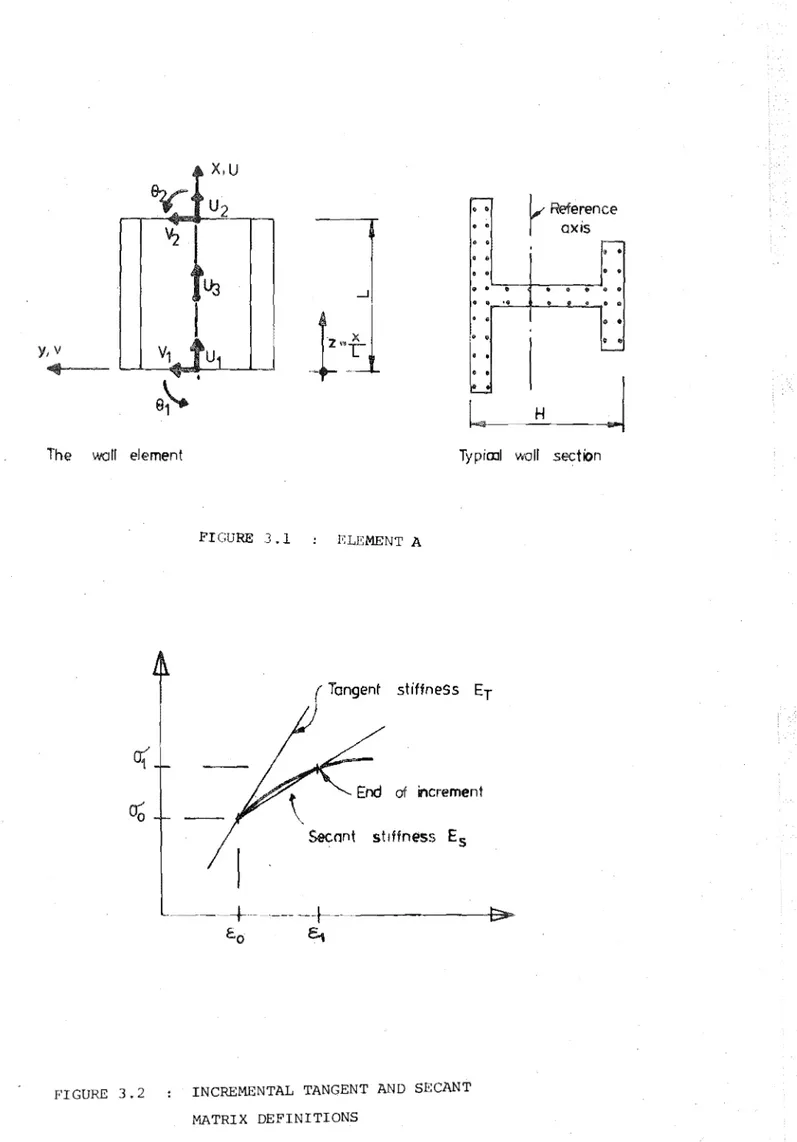
A suitable displacement function, based on a flexural idealisation, was specified to represent walls. The finite element model A (figure 3.1) is based on a pure displacement model [33]. Because the element is reduced to one dimension and only end connectivity is present, then equilibrium is not violated across the boundaries as is the case with many two-dimensional elements. The internal degree of freedom at the mid point (figure 3.1) was introduced in order that the strain variation due to axial deformation be of the same degree as the strain variation due to flexure. This allows non-coincidence of the incremental neutral axis and the reference axis to be recognised within the element. It is assumed in this chapter that

section properties at the required locations are available. The incremental stiffness of element A is derived using finite element techniques to

X,U

Y

•

•

r

~

t~

_l

· .

•

•

-•

•

•

• •

·

.

•

•

•

I

1-1

.

. .

·

.

..

.

';II V

•

•

_•

_•

V1

_•

e~'

The woll element Typiml wall section

FIGURE 3.2

FIGURE 3.1 _{ELEMENT A}

Tangent stiffness Er

End of increment

Secant stIffness Es

- ' - ' -4---

--t---t=:t;:..,...

E.o

€.t

3.5.2 Displacement Functions

The following standard expressions relate to figure 3.1. Symbol definitions are listed at the beginning of this thesis.

a) Axial displacement along element u u(z) - [N ]

u {U} (3.1 )

where [N ] (1 - z, z, 4z (l - z)] u

{ u } _{(u l ' u2 , u3]} T

z x/L and L is the beam length. b) Transverse displacement along element v

v( z) [N J {v} (3 .2)

v

where [N ] _v [1 - 3z 2 + 2z , Lz(l - z) , 3 2 1 - 3(1 - z) 2 + 2(1 . )3 - z - L z 2 ( 1 - z) ] and {v} = _[vI' 8 , v T

2 ,82 ]

1

c) Combined displacement function N

[uez) ]

_[:u

:J

[:]

{u(x,y) } = = [N] {q}

v( z)

v

(3.3)

where {q} is the nodal displacement vector. 3.5.3 Element strains

Utilising Kirchhoff's hypothesis and assuming a uniaxial stress state, the strain {E} within the element is expressed as follows:

(x,y) }

~aN

aN

~

~

_{_.Y}

dzv {q} L dz _L2

= [B] {q} (3.4)

PI'dorming the differentiations in equation 3.4 and substituting x = Lz gIves the strain displacement relationship (B] as a function of position.

[8] =

[-

L L 2

L

3X)J

2Y ,_ 2Y(L - _(3.5)

This is the basic strain displacement relationship which is used to compute material strains at sections as the analysis progresses.

3.5.4 Constitutive Relationships

In physically nonlinear problems the material properties vary as functions of deformation and deformation history. An important aspect of the analysis is, therefore, the definition of stress-strain curves or

constitutive relationships. At every stage of an iterative or incremental procedure, new element stiffness matrices must be computed and a prerequisite

to this computation is the knowledge of current values of the material parameters [C]. Inelastic deformation is characterised by irreversible straining and is governed by a yield criteria of the form

F (

{oJ ,

which must be defined. The actual relationships, together with consideration of the two material composition of reinforced concrete, are dealt with in Chapter 4.

stress

{oJ

In general, however, if

{o}

o 0

and strain {£} values at the end of the previous increment then [C (x,y)] , the tangent constitutive matrix, may be defined.

o

{oJ

0 0 0 (3.7)

The terms

{oJ

conventional elastic analysis procedures apply and overall solutions comprise cumulative results. Since a state of plane uniaxial stress is assumed in this s·tudy and ET is the Young's Modulus of the material computed at the commencement of an increment (tangent modulus), the following simplification is possible

(3.8)

Because of departures from linearity, actually resisted stresses {Ol}' as distinct from stresses predicted in the linearised equation 3.7, must be computed at the end of the increment.

[C (x,y)] de} - {£ }) + {o }

S 0 0 (3.9)

wlwn~ rc£; (x,y) 1 is the local secant constitutive matrix. If Es is

3.8, is possible, i.e. [C ]

s [E ] s (3.10 )

l x l

The secant and tangent moduli are illustrated in figure 3.2. 3.5.5 Energy Solution for a Single Element

A generalised method of computing the element stiffness matrix is to apply one of the variational principles of solid mechanics. Usually, when a compatible displacement element is considered, the principle of minimum potential energy is selected and i t is used in the following derivation.

For a linearised increment, where {6Se} is the vector of incremental nodal forces associated with one element, the potential energy may be written in its general form, i.e.

u

; [

I

dEl -

do} -

- T .

- {q} {Me}]

where

{q}

-and U is the strain energy associated with the increment.

By substitution into equation 3.11 from 3.4 and 3.7, it follows that:

=

; [ I

(3.11)

- T

- {q} {6Se}] (3.12)

Applying the principle of minimum potential energy, where

{oq}

Vol

[B] T [C ] [BI d Vol {q} o

ill1d since

{oq}

J

o {Me}

Vol

o

-By definition, the 7 x 7 incremental stiffnoss ma.trix [K] is given u;; follows:

::::

f

Vol 7 x l I x l I x 7

(3.15)

The detailed evaluation of this integral is discussed in section 3.5.7. Formation of the total stiffness matrix is achieved using direct stiffness methods as described in section 3.9.

3.5.6 Force Computation

On completing the increment, predicted elastic forces {So} are easily computed using equation 3.14, since the integral has been evaluated previously. Strictly, the actual nodal forces {Sr} should be computed by substitution of [C ]

s for [C] o in equation 3.14 and re-evaluation of the integral. However, for this particular element, considerable

simplification is possible because of "end only" connectivity. Actual stress distributions may be simply integrated across boundary sections as outlined in Chapter 4, with the resultants expressed as standard beam actions.

3.5.7 Evaluation of Element A stiffness

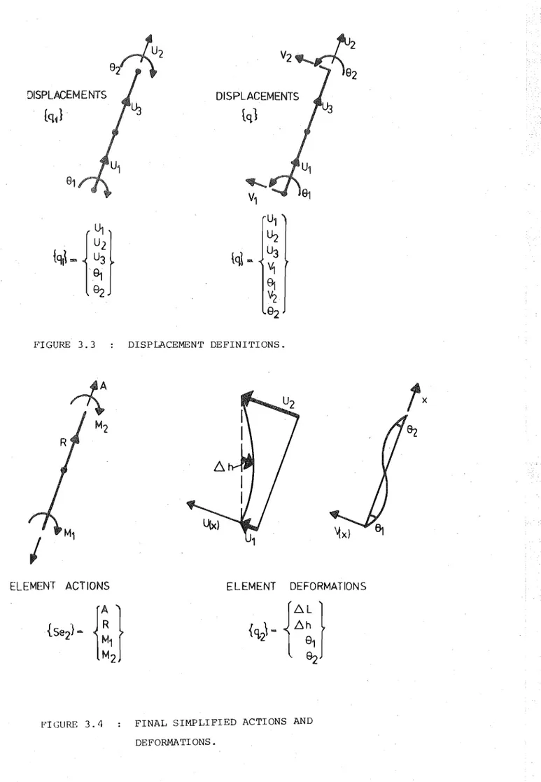
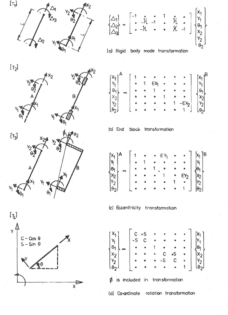
In the interests of computational efficiency the numerical stiffness matrix operations within the program have been streamlined as much as possible. For instance, in transforming stiffness matrices to global systems, it is advantageous to operate on,the minimum dimension stiffness matrix, obtained by eliminating rigid body modes. Transformation

[TS1, relating to figure 3.3, is useful in this respect and the resulting degrees of freedom are still adequate to define curvature and axial

strain deformation patterns. Transformation [TS] is defined as follows:

u

l 1

r

1

\1

2 1 u2

i

u

3 1

I _u

3 (3.16)

I

1 1 I

~l -1 0

i

v,

L L

() ')

1 1

1 0

l8

..

v 2 8₂

FIGURE 3.3

I

DISPLACEMENT DEFINITIONS.

ELEMENT ACTIONS ELEMENT DEFORMATIONS

{Se2)-

gJ

h21-

{~~}

Further, defining a new strain displacement relationship [B

l ) in equation 3.17 and combining with the original strain displacement relationship of equation 3.4 gives

{E:}

{d

[B l )

On performing the matrix

[ _ 1

L " L 1

[B

l ] {ql}

[B) {q} [B) [T J T

5

multiplication

4 (L - 2x) L2

[B

l ] is obtained

- 2y(2L - 3x) L2

(3.17)

(3.4)

(3 . 18)

] (3.19)

The two constant components of equation 3.19 may be combined using the definitions of figure 3.4. A new length parameter 6L expressing element elongation is used.

(3.20)

The middle node displacement is redefined, where 6h is defined as shown in figure 3.4.

6h

and the final strain displacement relationship [B

2) is derived.

1 4 (L - x) L ' L2

- 2y (2L - 3x) L2

- 2y(L - 3x) ] L2

(3.21)

(3.22)

ibis departure from specifying all parameters, as is usual in the finite element method, in terms of nodal displacements or derivations of

displacements, Is possible in this case only because of the simplified nature of [Bll.

The stiffness matrix [K

2J , relating to displacements {q2} of figure 3.4, may be expressed in integral form as follows:

[K

21 =

J

[B

2] d Vol (3.23)

4x4 Vol 4xl lx4