Flexible Model Selection Criterion for Multiple Regression
Kunio Takezawa
National Agriculture and Food Research Organization, Agricultural Research Center Graduate School of Life and Environmental Sciences, University of Tsukuba, Tsukuba, Japan
Email: [email protected]
Received July 17,2012; revised August 20, 2012; accepted August 31, 2012
ABSTRACT
Predictors of a multiple linear regression equation selected by GCV (Generalized Cross Validation) may contain unde-
sirable predictors with no linear functional relationship with the target variable, but are chosen only by accident. This is because GCV estimates prediction error, but does not control the probability of selecting irrelevant predictors of the
target variable. To take this possibility into account, a new statistics “GCVf” (“f” stands for “flexible”) is suggested. The
rigidness in accepting predictors by GCVf is adjustable; GCVf is a natural generalization of GCV. For example, GCVf is
designed so that the possibility of erroneous identification of linear relationships is 5 percent when all predictors have no linear relationships with the target variable. Predictors of the multiple linear regression equation by this method are highly likely to have linear relationships with the target variable.
Keywords:GCV; GCVf; Identification of Functional Relationship; Knowledge Discovery; Multiple Regression;
Significance Level
1. Introduction
There are two categories of methods for selecting pre- dictors of regression equations such as multiple linear regression. One includes methods using statistical tests such as the F-test. The other one includes methods of
choosing predictors by optimizing statistics such as GCV
or AIC (Akaike’s Information Criterion). The former
methods have a problem in that they examine only a part of multiple linear regression equations among many applicants of the predictors (e.g., p. 193 in Myers [1]). In this point, all possible regression procedures are desirable. It has spread the use of statistics such as GCV and AIC to
produce multiple linear regression equations.
Studies of statistics such as GCV and AIC aim to con-
struct multiple linear regression equations with a small prediction error in terms of residual sum of squares or log-likelihood. In addition, discussion on the practical use of multiple linear regression equations advances on the assumption of the existence of a linear relationship between the predictors adopted in a multiple linear re- gression equation and the target variables. However, we should consider the possibility that some predictors used in a multiple linear regression equation have no linear relationships with the target variable. If we cannot ne- glect the probability that some predictors with no linear relationships with the target variable reduce the pre- diction error by accident, there is some probability that one or more predictors with no linear relationships with
the target variable may be selected among the many applicants of predictors. Hence, if our purpose is to select predictors with linear relationships with the target va- riable, we need a method different from those that choose a multiple linear regression equation yielding a small prediction error. We address this possibility in the following discussion.
We present an example that casts some doubt on the linear relationships between the predictors selected by
GCV and the target variable in Section 2. In preparation
to cope with this problem, in Section 3, we show the association between GCV (or AIC) and the F-test. In
Section 4, on the basis of this insight, we suggest “GCVf” (“f” stands for “flexible”) to help solve this problem.
Then, in Section 5, we propose a procedure for estimating the probability of the existence of linear relationships between the predictors and the target variable using GCVf.
Finally, we show the application of this method to the data which is used in Section 2.
2. Definition of the Problem Using Real Data
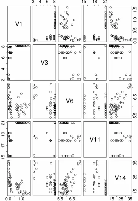
We use the first 50 sets of Boston house price data (named “Boston”) retrieved from StatLib. These data consist of 14 variables. The applicants of the predictors ({x1, x2, x3,
x4}) and the target variable (y) are selected among them:
x1: per capita crime rate by town;
x2: proportion of nonretail business acres per town;
x3: average number of rooms per dwelling;
x4: pupil-teacher ratio by town;
[image:2.595.60.290.218.327.2]y: median value of owner-occupied homes in $1000’s.
Figure 1 shows a matrix of scatter plots for showing
the distributions of the above data. The correlations of the target variable with x1 and x3 appear to be high. The
negative correlation between x1 and y indicates that house
prices in crime-ridden parts of the city tend to be low. The positive correlation between x3 and y implies that
house price is relatively high if the average number of rooms per household in an area is large. The result of the
Coefficients:Estimate Std.Error t value Pr
t(Intercept) −28.0049 10.6679 −2.625 0.01179*
x.1 −6.7668 1.6640 −4.067 0.00019***
x.2 −0.5825 0.3324 −1.752 0.08651 x.3 7.3779 1.1860 6.221 1.47e−07***
x.4 0.5784 0.3121 1.854 0.07037 Signif.codes: 0“***”0.001; “**”0.01; “*”0.05; “.”0.1; “ ”1
Residual standard error: 2.841 on 45 degrees of freedom Multiple R-squared: 0.7957, Adjusted R-squared: 0.7776 F-statistic: 43.83 on 4 and 45 DF, p-value: 5.692e−15.
Figure 1. Matrix of scatter plots using four applicants of predictors and the target variable. The first 50 sets of Boston house price data (named “Boston”) are used.
construction of a multiple linear regression equation using 50 datasets with all the predictors is shown below. The R command lm() installed by default was used for this purpose.
The above table shows that {x1, x3} should be chosen
as predictors if a 5 percent significant level is adopted in the t-test.
However, if predictors are not independent of each other, this result is not necessarily reliable. Then, all possible regression procedures using GCV were carried
out to select predictors. GCV is defined as
2,1 1
RSS q GCV q
q n
n
20 1
if 0
n
i i
RSS q y a q
(1)
where n is the number of data and q is the number of
predictors. RSS(q) is
0 21 1
if 1,
q n
i j ij
i j
RSS q y a a x q
(2where {xij} indicate the data of the selected predict
orrect, the data ({y}) of
th
1 50
i
y i . The
n unchanged. Th
wn in Figure 2 where the frequencies
of
)
ors. {aj} are regression coefficients given by conducting the
least squares using selected predictors. {yi} shows the data
of the target variable. The above procedures were uses to select all predictors ({x1, x2, x3, x4}). Predictor selection
by GCV results in a multiple linear regression equation
that is expected to provide a small prediction error with the use of the regression equation for predictive purposes. Hence, since the multiple linear regression equation using {x1, x2, x3, x4} is of great use for prediction, we are
inclined to think that each of the predictors {x1, x2, x3, x4}
has a linear relationship with y.
To determine whether this is c i
e target variable (y) are randomly resampled with
replacement to obtain n data
B
data of the target variable remai e pro-
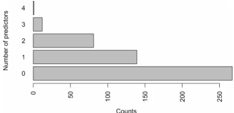
cedure was repeated 500 times while varying the seed of the pseudo-random number generator. This procedure provided 500 sets of bootstrapped data. The values of the target variable of these bootstrapped data are provided by random sampling from a population with a distribution given by the data of the target variable; hence, they are not associated with the predictors. Therefore, if pre- dictors are selected using these bootstrapped data, a con- stant seems to be almost always chosen as the best re- gression equation.
The result is sho
[image:2.595.61.284.372.696.2]Figure 2. Frequencies of the number of predictors selecte
the data do not have linear relationships between the
e predictors are chosen by all possible re
3. Relationship between Model Selection
F(
d by GCV.
if
predictors and the target variable, a functional relation- ship represented by a multiple linear regression equation or a simple regression equation is found at about 50 per- cent probability.
Therefore, if th
gression procedures using statistics such as GCV, we
should not rule out the possibility that they contain one or more predictors with no linear relationships with the target variable. This implies that we need a new model selection criterion. This new criterion should choose predictors only if the predictors are highly likely to have linear relationships with the target variable.
Criterion and F-Test
n, q)(F values) is defined as
1
RSS q
1 ,
1 1
1 1 .
RSS q F n q
RSS q n q RSS q n q RSS q (3)
Hence, we have
1 , 1. 1
F n q
RSS q n q
(4)
Furthermore, Equation (1) leads to RSS q
2 2 1 1 1 1 q n q n (5)The substitution of Equation (4) gives
1 RSS q GCV q GCV q RSS q
1 ,GCV q F n q n 2
2
1 .
1 1 1
q
GCV q n q n q (6)
Therefore, when we have a multiple linear regression equation with (q – 1) predictors, the condition f
ing a q-th predictor is written as
or accept-
1 2 2 , 1 1. 1 1F n q n q
n q n q
(7)
That is,
,
2 1 .
1
n q
F n q n q
n q
(8)
[image:3.595.322.541.128.210.2]If the inequality sign in the above equation is replaced with an equality sign and n = 25, F(n,
Figure 3 (left panel). This shows that when we use GCV, F(
q) is shown as in n, q) for determining whether the q-th predictor should
be added to the multiple linear regression equation with (q – 1) predictors is nearly independent of q.
If the multiple linear regression equation with (q – 1)
predictors is correct, F(n, q) is written as
R2
q R
2
q1
1, 1 2 , ~ . 1 1 n q
F n q F
R q n q (9)
1,n q 1
F stands for the F distribution; the fi
of freedom is 1 and the second degree of freedom is (n – q – 1). R2(q) is the coefficient of determination defined as
rst degree
2
1 1 2 2 1 ˆ , j n n q i j y y n
R q
(10)1 1 1 j n n i i j y y n
where
ˆ q iy are estimates derived us
linear regression equation with q predictors. Then, we
calculate p that satisfies the equation
where den(1, n – q – 1, x) is the probability density
function of an F distribution; the first degree
is 1 and the second degree of freedom is (n – q –1). p is
ing a multiple
,
1, 1, d ,
F n q
p den n q x x
(11)of freedom
the value of the integral. The lower limit of the inte- gration of the probability density function with respect to
x is F(n, q, p). This p represents the probability that F is
larger than F(n, q) when the multiple linear regression
function with (q – 1) predictors is a true one. Hence, the
values of F(n, q) drawn in Figure 3 (left panel) are sub-
stituted into Equation (11); the resultant values of p are
shown in Figure 4 (left panel). These values of p are the
probability that the q-th predictor is wrongly accepted
when the multiple linear regression equation with the (q –
1) predictors is correct. That is, this is the probability of a type one error. When the forward and backward selection
Figure 3. Relationship between q and F(25, q) corresponding to GCV and AIC.
Figure 4. Relationship between q and p corresponding to GCV and AIC (n = 25). method using F valu
xed at values ranging from 0.25 to 0.5 (e.g., p. 188 in
linear regression eq
e is carried out, this probability is fi
Myers [1]), or 0.05 (e.g., p. 314 in Montgomery [2]). Therefore, the selection method for predictors by GCV
has similar features with the forward and backward selection method with a fixed p because p in Figure 4
(left panel) is nearly independent of q.
On the other hand, the forward and backward selection method does not compare the multiple
uation with predictors of {x1, x2} with that with
predictors of {x3, x4} for example. This type of com-
parison can be performed by GCV. All possible regres-
sion procedures using GCV entail such a comparison.
Hence, the comparison of two multiple linear regression equations in the forward and backward selection method should be on par with that of the same multiple linear re- gression equations by all possible regression procedures.
On the other hand, AIC is defined as
log 2
π logAIC q n n
n
2 4.
n q
Hence, we have
RSS q
(12)
1
log RSS
AIC q AIC q n
1
log 2 log
1
q n
RSS q RSS q
n n
n RSS q
2.
(13)
The substitution of Equation (4) leads to
11
,
log 1 2 0.
1
AIC q F n q n
n q
AIC q
(14)
Therefore, if we have a multiple linear regression equation with (q −1) predictors, the condition for accept-
in
g a q-th predictor is
1
, 1 exp 2 . 1
F n q
n q n
That is,
(15)
, 1 exp
2 1 .F n q n q
n
n in this equation is replaced with an equality sign, F(n, q) (n = 25) is drawn in Figure 3
(16)
(left panel). The corresponding p is shown in Figure 4
(right panel). It shows the characteristics
show that, when we have a multiple linear regression eq th (q − 1) predictors, p for determining whether
to accept a q-th predictor augments with an increase i
This is consistent with the tendency that AIC
new predictor with comparative ease when the present
he q-th predictor when the following
equation is satisfied:
of AIC which
uation wi
n q.
accepts a
multiple linear regression equation has many predictors.
4. Introduction of GCV
fIn the previous section, we associate GCV and AIC with
the forward and backward selection method using F. This
indicates that GCV is desirable as long as p is nearly
independent of q. However, if p corresponding to a
model selection criterion should be independent of q, we
may well develop a new model selection criterion that meets the requirement. Then, if p is given, F(n, q, p) is
calculated using
, ,
1, 1, d .
F n q p
p den n q x x
(17)The difference between Equations (17) and (11) is that Equation (11) is used to obtain p when F(n, q) is given,
whereas Equation (17) works as an equation for calculating
F(n, q, p) when p is in hand. Equation (4) indicates that
the multiple linear regression equation with (q − 1) pre-
dictors accepts t
1 , ,
1.
RSS q F n q p
(18) 1
RSS q n q
Therefore, we suggest the following GCVf(q) as a new
model selection criterion:
if 02
f
RSS q
GCV q q
n
1 , , 2 q f k1 if 1. 1
F n k p
GCV q q
n n k
(19)This criterion is justified because it is a criterion in w
-th predictor is depicted as Eq on (18) (q1). Hence, GCVf(q), a new model
criterion, is the same in function t e forward and backward selection method using the F-test with a p
significant level in determining whether or not a q-t
dictor is accepted. GCVf(q) stands for “flexible GC
discussion on model selection, the focus is on choosing be
rdin RSS q
hich a multiple linear regression equation with (q − 1)
predictors accepting a q
uati
selection o th
h pre-
V”. In
tween GCV and AIC, for example. However, GCVf(q)
allows us to adjust the characteristics of the model selection criterion continuously by varying p. Therefore,
if p is tuned acco g to the nature of the data or to the
purpose of the regression, we have an appropriate model
selection criterion. The background that made us think of
GCVf(q) as a flexible version of the conventional GCV(q)
is as follows.
Let the coefficient of RSS q
n in GCV(q) (Equation (1)) be CGCV(q). Then, we have
1 2.1 1 CGCV q q n (20)
Let the coefficient of RSS q
n in GCVf(q) (Equation (1
9)) be CGCVf(q). Then, we have
1 , , 1 . f k k p CGCV qn n k
2 q F n
n
1
(21)when n is large, the equation below holds:
, , 0.1573
, , 0.1573
2.0.F n q F q (22) Thus, if q1 and p = 0.1573 are satisfied, we obtain
2 2 21 1 1 CGCV q q q n n n
(23)
1 1
2 2 1 q ,
1 1 1 f k CGCVn n k
1 , ,0.1573 2 2 2 1 1
2 2 2 2 1 1 1 .
q
q k
F n k n
q
n
n n k
q q
n n n
(24)If q = 1, we have
21 2
1 1 .
1 1 CGCV n n (25) 2 1 . f CGCV n
(26)
tions (23)-(26), GCVf(q) is appro-
xim GCV(q) when p = 0.1573.
Because of Equa ately identical to
CGCV(q) and CGCVf(q) when n
shown in Figure 5. It demonstrates th
= 0.1573 is set are approximately identical to those of GCV(q). Furthermore, a small p is assumed in CGCVf(q);
CGCVf(q) is large. This indicates that GCVf(q) with a
small p selects a multiple linear regression equation with = 100 are set are
at GCVf(q) when p
Figure 5. CGCV(q) and CGCVf(q). “ × ” CGCV(q), “”
CGCVf(q) (p = 0.05), “〇” CGCVf(q) (p = 0.1573), “”
CGCVf(q) (p = 0.5).
a small number of predictors.
5. Identification of Linear Functional
Relationships Using GCV
fThe discussion in the previous section shows that GCVf(q)
enables us to adjust the rigidness of accepting new o
s
f the targ
predictors. By taking advantage of this feature, a meth d of including predictors with a clear causal connection is developed. This method i performed as follows:
1) Let the data o et variable be yi
1 i n
.acement from
{y}. The
procedure ispseudo-
ran of predictors remain
riginal data.
ese bo
probability. This in- di
rcent si
n data are randomly resampled
B
with repl
y 1 i n
. Thei i
repeated 500 times by varying the seed of the dom number generator. The data
n, we have
unchanged. Thus, we have 500 sets of bootstrapped data. 2) Using various values of p, predictors are selected by GCVf(q); this process is carried out for 500 sets of boot-
strapped data. We choose p by which the probability of
obtaining regression equations except a constant one is approximately 0.05.
3) Using p selected in (2), model selection by GCVf(q)
is carried out for the o
This method generates sets of bootstrapped data of which the data of the target variable are resampled ones; hence, there is no causal connection at all between the data of the predictors and those of the target variable. This is because the values of the target variable are sam- pled from a population with a distribution given by the data of the target variable; the values of the target varia- ble are not associated with those of the predictors. Al- though the predictor variables are selected using th
otstrapped data, regression equations except a constant may be produced with considerable
cates that the model selection criterion is very likely to accept predictors. Therefore, we should find p to make
this probability approximately 5 percent. When the model selection is carried out using GCVf(q) given by the op-
timized p, a regression equations except a constant will
be selected at a 5 percent probability when a constant should be chosen. This strategy quells our suspicion that a constant might be actually desirable even though regre- ssion equations except a constant were selected. This me- thod is similar to Generalized Cross-validation Test (p. 87, in Wang [3]) in which the Monte Carlo method is carried out to test whether a regression equation should be parametric such as a simple regression equation.
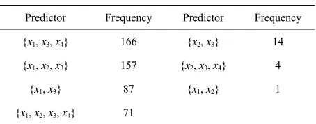
Next, model selection was carried out for the data used in Section 2. GCVf with various values of p was used for
choosing predictors that are highly likely to have linear functional relationships with the target variable; the data of the target variable were bootstrapped. Table 1 shows
the results using the settings of p = 0.01, p = 0.06, p =
0.05 and p = 0.04. When GCVfwith p = 0.05 is em-
ployed, a constant was selected in 446 sets. Hence, if a model selection method adopts GCVf with p = 0.05 and
multiple linear regression equation except a constant are chosen, we reject the null hypothesis at a 5 pe
gnificance level: there are no linear functional relation- ships between the predictors and the target variable. Then, a model selection by all possible regression procedures was carried out using GCVf with p = 0.05. GCVf is mini-
mized when {x1, x3, x4} were chosen. On the other hand,
a model selection by all possible regression procedures using GCV chose {x1, x2, x3, x4} in Section 2. In view of Figure 2, this result follows our intuition that one or
more predictors among the four selected ones may not have linear functional relationships with the target varia- ble.
However, if the data are slightly altered, GCVf with p
= 0.05 may choose different predictors from {x1, x3, x4}.
If this possibility is correct, the selection of {x1, x3, x4} is
not valid. To clarify this point, a bootstrap method in the usual sense is conducted for these data; 500 sets of boot- strapped data are generated. That is, the data set of {(xi1,
xi2, xi3, xi4, yi)} (1 i 50) was randomly resampled with
[image:6.595.309.537.630.734.2]replacement whereas the set of values of the predictors
Table 1. Frequencies of the number of selected predictors.
Number of predictors p = 0.1 p = 0.06 p = 0.05 p = 0.05
0 404 446 453 461
1 66 44 37 31
2 29 10 10 8
3 1 0 0 0
Copyright © 2012 SciRes. OJS
and the target variable was w ped. When model selec- t
dat 2. { , x r
1 a 1 2 3 s d
fo 157 datasets. The re, x3, x not only
c ce as a set of pred rs w ear relations with
the target variable. {x 2, x3 possible choice
w n we proceed wit e dis ion o is dat
6. Conclusions
func- with the target variable are contained the predictors, one or more such pre-
rap
ion by GCVf with p = 0.05 was carried out for 500
asets, we obtained 66 datasets. On the
Table
other h
x1, x3
nd, {x, x
4} was cho
, x} wa
sen fo selecte
r refo {x1, 4} is the
hoi icto
, x
ith lin } is also a
hips
1
h th
he cuss n th a.
We have assumed that when GCV or AIC yields a
multiple linear regression equation with a small predic- tion error, there is a linear functional relationship be- tween the predictors employed in the regression equation and the target variable. Not much attention has been paid to the probability that one or more selected predictors actually have no linear functional relationships with the target variable. However, we should not ignore the pos- sibility that when several predictors with no linear tional relationships
in the applicants of
dictors are adopted as appropriate predictors in a multiple linear regression equation. This is because when many applicants of the predictors have no linear relationships with the target variable, one or more such predictors will be selected at a high probability, since p in Figure 4 does
[image:7.595.59.286.536.625.2]not depend on the number of applicants of the predictors. Hence, another statistics for model selection based on an approach different from the use of prediction error is required for choosing predictors with linear relationships with the target variable. The new statistics should make the threshold high for accepting predictors when quite a few predictors have no linear functional relationship with the target variable. Although this strategy poses a re- latively high risk of rejecting predictors that actually
Table 2. Frequencies of selected predictors.
Predictor Frequency Predictor Frequency {x1, x3, x4} 166 {x2, x3} 14
{x1, x2, x3} 157 {x2, x3, x4} 4
{x1, x3} 87 {x1, x2} 1
{x1, x2, x3, x4} 71
hav ationshi ith the t ariable, we have
to accept this trade-off. T is policy is quite similar to that
of m omparis n wh cept th com-
parat gh risk of ing n nce when there
is fferenc ith the purpose of reducing the
[2] D. C. Montgomery, E. A. Peck and G. G. Vining, “In-
troduction to ysis,” 3rd Edition,
Wiley, New Y
e linear rel ps w arget v
h on i
ultiple c ich we ac e
ively hi detect o differe
actually a di e w
risk of mistakenly finding a difference when there is no difference.
Using the statistics of GCVf suggested here, we select
one or more predictors at a 0.05 probability when no predictors have linear relationships with the target varia- ble. If we select predictors using this new statistics, the chosen predictors are less likely to contain those that have no linear relationships with the target variable.
However, there is still room for further study of the detailed characteristics of GCVf produced by the pro-
cedure presented here. In particular, we should know the behavior of GCVf when there are high correlations
between predictors.
The discussion so far indicates that the criteria for se- lecting predictors of a multiple linear regression equation are classified into two categories: one aims to minimize prediction error and the other is designed to select pre- dictors with a high probability of having linear relation- ships with the target variable. GCV and GCVf are exam-
ples of both categories, respectively. Interest has been focused on the derivation of multiple linear regression equations yielded using a criterion of prediction error. We expect that more attention will be paid to the prob- ability of the existence of linear relationships. Further- more, we should study whether a similar discussion is possible with respect to regression equations different from the multiple linear regression equation.
REFERENCES
[1] R. H. Myers, “Classical and Modern Regression with Applications (Duxbury Classic),” 2nd Edition, Duxbury Press, Pacific Grove, 2000.
Linear Regression Anal ork, 2001.