Development of a two stage inspection process for the assessment of deteriorating infrastructure

www.elsevier.com/locate/ress

Author’s Accepted Manuscript

Development of a two stage inspection process for

the assessment of deteriorating infrastructure

Emma Sheils, Alan O’Connor, Denys Breysse, Franck

Schoefs, Sylvie Yotte

PII:

S0951-8320(09)00228-2

DOI:

doi:10.1016/j.ress.2009.09.008

Reference:

RESS 4226

To appear in:

Reliability

Engineering

and

System Safety

Received date:

9 February 2009

Revised date:

17 September 2009

Accepted date:

27 September 2009

Cite this article as: Emma Sheils, Alan O’Connor, Denys Breysse, Franck Schoefs

and Sylvie Yotte, Development of a two stage inspection process for the

as-sessment of deteriorating infrastructure,

Reliability Engineering and System Safety

,

doi:

10.1016/j.ress.2009.09.008

Accepted manuscript

Development of a two stage inspection process for the assessment of

deteriorating infrastructure

Emma Sheils

, Alan O’Connor

, Denys Breysse

, Franck Schoefs

, Sylvie Yotte

1_{Deptartment of Civil Engineering, Trinity College Dublin, Dublin 2, Ireland}

*_{Corresponding Author: Tel: +353-1-896-1822, Fax: +353-1-677-3072, email: [email protected]}

2_{Université Bordeaux 1, GHYMAC, Bordeaux, France.}

3_{GEM, Université Nantes, Nantes, France.}

Abstract

Inspection based maintenance strategies can provide an efficient tool for the management of ageing infrastructure

subjected to deterioration. Many of these methods rely on quantitative data from inspections, rather than qualitative

and subjective data. The focus of this paper is on the development of an inspection based decision scheme,

incorporating analysis on the effect of the cost and quality of NDT tools to assess the condition of infrastructure

elements/networks during their lifetime. For the first time the two aspects of an inspection are considered, i.e.

detection and sizing. Since each stage of an inspection is carried out for a distinct purpose, different parameters are

used to represent each procedure and both have been incorporated into a maintenance management model. The

separation of these procedures allows the interaction between the two inspection techniques to be studied. The

inspection for detection process acts as a screening exercise to determine which defects require further inspection for

sizing. A decision tool is developed, which allows the owner/manager of the infrastructural element/network to

choose the most cost efficient maintenance management plan based upon his/her specific requirements.

Accepted manuscript

1. Introduction

Due to the extent of deteriorating infrastructure in the U.S. (about 5,000 bridges become classed as deficient each

year), the estimated cost of rehabilitation and repair has been estimated at $1.3 trillion [1]. “The federally mandated

biennial inspection interval is not the most cost-effective maintenance strategy for bridges [2], and bridge repairs are

not always performed with life-cycle cost effectiveness in mind” [1]. As a result, over the last decade a lot of

research has been conducted into optimisation of the existing infrastructural resource to develop methods of

maintenance management which consider the dual constraint of optimal maintenance budget while maximising

efficiency for the required remaining service life [3, 4, 5, 6, 7, 8, 9, 10, 11 12, 13, 14, 15, 16]. The main objective is

to find the optimal maintenance management plan, thereby optimizing the life-cycle cost of the structure. Many of

these methods rely on quantitative data from inspections, rather than qualitative and subjective data. Consequently,

monitoring and inspections are key aspects in this process [17] as the information from these tests can be used to

update deterioration models and to derive the optimal economic maintenance strategy for the remaining lifetime of

the structure.

The main focus of this paper is on the development of an inspection based decision scheme, incorporating analysis

of the effect of the cost and quality of NDT tools to assess the condition of infrastructure elements/networks over

their lifetime. Two aspects of an inspection, i.e. detection and sizing are considered here. The aim is not to compare

existing strategies but to suggest a new systematic approach which facilitates quantification of cost and predicts the

required maintenance budgets as a function of time. There have been many studies which focus only on the

detection stage of an inspection, using various sets of parameters such as Probability of Detection and Probability of

False Alarm [18, 19], Probability of Detection and Probability of False Indications [20] or Probability of Detection

and False Call Probability [21, 22] to assess the quality of a particular inspection method. In this study a distinction

has been made between an inspection carried out to detect a defect, and an inspection carried out to size a defect.

Since each stage of an inspection is carried out for a distinct purpose, different parameters are used to represent each

procedure and both have been incorporated into a maintenance management model. By separating these two

Accepted manuscript

technique for each stage of the inspection, whether it is for detection or sizing, rather than using the same inspection

technique for both procedures.

As part of the new process the first part of an inspection is concerned with the detection of existing defects. The

Probability of Detection (PoD) and the Probability of False Alarm (PFA) are used in this study, for a particular NDT

tool used in the assessment, to indicate the quality of the inspection method for detection. The second part of an

inspection deals with the assessment of the size of the defect knowing that it has already been detected. For this part

of the analysis, two new parameters are introduced, Probability of Good Assessment (PGA) and Probability of

Wrong Assessment (PWA). In this context it has been necessary to introduce a distinction between good and wrong

sizing assessments that lead to repair (PGAR, PWAR), and those which lead to no repair (PGANR, PWANR).

Using the methodology developed in Rouhan and Schoefs [19], an events based decision theory is subsequently

introduced to look at the effects of an individual good/bad inspection performance. Based on the inspection results,

for detection or sizing, a decision is made whether a further inspection should be carried out, or to repair. For

evaluating the cost of the system, and to find the optimum costs, it is useful to investigate whether the decision to

carry out a sizing assessment or a repair is correct/incorrect. On this basis, a decision scheme is introduced which

considers four inspection events for each of the two stages of an inspection. The probability of these events are

evaluated using Bayes Theorem and are subsequently introduced as parameters into cost functions which are used to

investigate the effect of cost overrun due to inaccurate inspection results.

In addition to this, for a particular set of input parameters the optimum time between inspections, which results in

the lowest annual cost, is determined. By varying the quality of the inspection techniques, the sensitivity of the

optimal inspection time to changes in the modelled parameters is assessed, allowing the optimum combination of

techniques to be determined for the constraint of optimisation of performance with respect to available budget.

The purpose of this study is to develop a method which simulates the deterioration, inspection, repair and failure of

structures over time using Markov matrices, with the ability to consider many different forms of defect growth and

Accepted manuscript

environments (i.e. passive and aggressive) and limit states (i.e. Ultimate, Fatigue and Serviceability) to be studied.

For example, this method can be used to simulate the deterioration and repair of a structure in a marine environment.

By varying the growth parameters, the effects of: (i) different environments (mild or aggressive) and concrete mixes

on the growth rate of the cracks and rate of spalling in reinforced concrete [15], (ii) corrosion-fatigue crack growth

in steels [23] or (iii) decay of timber structures [24] can be modelled. In all cases the optimum inspections

techniques for each stage of deterioration for each environment can be determined.

2.

Probabilistic Modelling of Inspection Results

When carrying out an inspection or any non destructive measurement, one has to consider measurement error

associated with the signal output from the measurement instrument. Measurement error is caused by imperfect

instruments, quality of the protocol (which is dependent on the inspector) and sample disturbance when a quantity is

observed. It generally involves two components: (i) a systematic error associated with the bias in the measurements,

and (ii) a random error associated with the precision in the measurements [25]. The precision of the measurement

depends on the equipment, on the expertise of the measurer and on the conditions (e.g. meteorology) during

measurement. This concept is also valid in the case of visual inspection, since the expert’s brain and eyes are no

more than a sensor. By knowing the true value and performing a statistical study, a distribution of noise is available.

The information obtained through inspection (e.g. cover depth, crack size etc.) is thus only an estimate of the true

reality (“signal of reference”), the difference between the two being due to bias and noise. Therefore, due to the

inherent uncertainty associated with inspections, many of the variables involved are modelled stochastically, and the

simulation of inspection results should be performed in a probabilistic sense. In the following, the systematic bias

will be neglected and only the noise will be considered.

For a given defect size, and the inspection method being used, there is a certain probability of detection [4, 26, 27].

On this basis, probabilistic methods are described below which are used to model inspection results for detection

and sizing assessment, taking this uncertainty into account. Note that the quantification of the on-site performance of

Accepted manuscript

field during the ICON project [28]. Other recent works provide data for the probability of detection of the corrosion

initiation in concrete [29, 30], the probability of detection and false alarm for uniform [31, 32] or localized [33]

corrosion of steel structures. Expert judgment can also be introduced in this regard [34].

2.1.

Stage 1 - Detection

It is assumed that every ΔT years, an inspection is carried out. The first part of an inspection is concerned with the

detection of existing defects. For an individual defect, it is assumed that detection of a defect by the first inspection

leads to a further inspection to assess the size of the defect, and that no detection leads to no further action. In this

study, the Probability of Detection (PoD) and the Probability of False Alarm (PFA) are the parameters chosen to

indicate the quality of an inspection method for detection and are used to assess if a defect will be detected or not

when an inspection is carried out, Figure 1. The PoD is the probability that a defect is detected by the inspection,

given that a defect is present, Equation 1, and the PFA is the probability that a defect is detected by the inspection,

given that no defect greater than the detection threshold is present, Equation 2.

PoD = P

(

)

PFA = P

(

)

The results of an inspection (and the ability of a method to detect a defect) depend on many different factors, such as

the NDT method, the detection threshold (dmin), the environment and several conditions of the structure [35], the

skill/experience of the operator, the characteristics of the defect (e.g. the deterioration mechanism such as

chloride-induced corrosion, fatigue etc.) and primarily on the size of the defect. For a given test, the PoD depends on the

defect size (for example the average defect size), the detection threshold and noise. The PFA, however, is

independent of the size of the defect and, depends only on the detection threshold and noise.

Therefore, the PoD is the probability that the signal “signal+noise” is greater than the detection threshold, dmin, and

the PFA is the probability that the signal “noise” is greater than the detection threshold [19]. For the general form of

Accepted manuscript

represents the error due to environmental conditions, human interference and the nature of what is being measured.

The distribution of signal represents the physical uncertainty of the inspection, and the distribution of the population

of defects at the time of inspection, Figure 1.

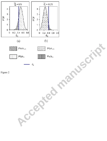
2.2.

Stage 2 - Sizing Assessment

The second part of an inspection deals with the assessment of the size of a defect. This assessment is only carried

out if the previous inspection has indicated that a defect exists. For this analysis, two new probabilities are defined,

the Probability of Good Assessment (PGA) and the Probability of Wrong Assessment (PWA). A repair of the defect

is carried out if the inspection indicates that the size of the defect is greater than the critical defect size dc. The value

of dc will be fixed by the owner/manager, depending on the safety level he/she wants to ensure. It can for instance be

related to the annual probability of failure. There is also a distinction made between good and wrong assessments

that lead to repair (subscriptR), and those which lead to no repair (subscriptNR), Equations 3-6.

(

)

R Pdˆ d |d d &dˆ d

PGA = ≥ ≥ ≥ (3)

(

)

NR Pdˆ d |d d &dˆ d

PGA = < < ≥ (4)

(

)

R Pdˆ d |d d &dˆ d

PWA = ≥ < ≥ (5)

(

)

NR Pdˆ d |d d &dˆ d

PWA = < ≥ ≥ (6)

Again, for this inspection, the accuracy of the results can depend on many different factors, and the noise can be due

to effects of environmental conditions, human interference and the nature of what is being measured. In this case

however, for a given inspection, both the PGA and the PWA depend on the defect size, the detection threshold and

noise. Therefore, the inspection can be modelled using just one distribution, as shown in Figure 2, where diis the

mean defect size within a group i. The PGAR is the probability that the “signal+noise” is greater than the critical

defect size (leading to repair), given that the actual defect is greater than the critical defect size dc, Figure 2(a), and

the PGANR is the probability that the “signal+noise” is less than the critical defect size (leading to no repair), given

Accepted manuscript

“signal+noise” is greater than the critical defect size (leading to repair), given that the actual defect is less than the

critical defect size, Figure 2(b), and the PWANR is the probability that the “signal+noise” is less than the critical

defect size (leading to no repair), given that the defect is greater than the critical defect size, Figure 2(a). An

example of the interaction between PGAR, PWAR, PGANR, PWANR and the critical defect size is illustrated in Figure

3.

3.

Events Based Decision Theory

As described in Rouhan and Schoefs [19], an events based decision theory can be used to look at the effects of a

good/bad inspection performance. Since there can be various sources of error when performing an inspection, it is

useful to investigate the probability that each of the decisions taken (e.g. to carry out a further assessment for sizing

or to repair) are correct/incorrect. In this study, a similar method is implemented for detection and sizing,

considering four inspection events for each of the two stages of an inspection. The probability of these events are

evaluated using Bayes Theorem and are subsequently introduced as parameters into cost functions which are used to

investigate the effect of cost overrun due to inaccurate inspection results.

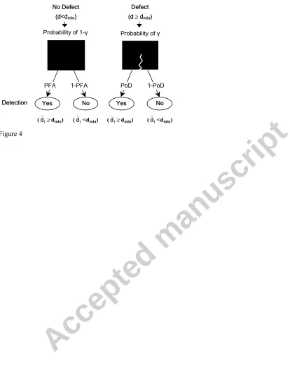
Firstly, in the case of an inspection to detect a defect, a decision on whether to carry out a further assessment is

made based on the inspection result dˆ1. It is assumed that detection of a defect by the first inspection leads to a

further inspection to assess the size of the defect, and that no detection leads to no further action. This decision on

whether or not to carry out a further assessment can never be taken with certainty, and the level of uncertainty

depends on the quality of the inspection and the level of the other sources of noise associated with the inspection. To

assess this risk, four events are defined for the detection stage of an inspection, labelled E1D, E2D, E3D and E4D

respectively. The question is, knowing that something is detected or not detected, what is the probability that there is

Accepted manuscript

• E1D is associated with a good decision, where the inspection indicates that there is no defect, when no

defect greater than the detection threshold (dmin) actually exists, in which case no further sizing assessment

is carried out, Equation 7.

( )

(

)

P = < < (7)

• E2D is associated with a bad decision, where the inspection indicates that there is a defect, when no defect

greater than the dmin actually exists, in which case an unnecessary sizing assessment is carried out, with an

associated inspection cost, Equation 8.

( )

(

)

P = < ≥ (8)

• E3D is also associated with a bad decision, where the inspection indicates that there is no defect, when a

defect greater than the dmin actually exists, in which case no sizing assessment is carried out, but there is an

associated failure risk cost, Equation 9.

( )

(

)

P = ≥ < (9)

• E4D is associated with a good decision, where the inspection indicates that there is a defect, when a defect

greater than the dmin actually exists, in which case a necessary sizing assessment is carried out, resulting in

an associated optimal spend, Equation 10.

( )

(

)

P = ≥ ≥ (10)

The calculation of these probabilities is based on the PoD, PFA and on the parameter γ, which is defined as the

probability that the actual defect size is greater than the detection threshold, Equation 11. This process can be

understood with reference to Figure 4.

(

)

P ≥

=

γ (11)

Accepted manuscript

( )

(

(

) (

)( )

)( )

P 1D − − + − − − = (12)

( )

( )

( )

P 2D

− +

−

= (13)

( )

(

(

) (

)

)( )

P 3D − − + − − = (14)

( )

( )

P 4D

− +

= (15)

3.1.

Events at Stage 2 – Sizing Assessment

For consistency in sizing assessment, the same methodology is employed. It is assumed that a repair is carried out if

the size of the defect from the second inspection (dˆ2) is larger than the critical defect size, dc, and that no repair is

carried out if the defect size is smaller than dc. Again, this decision on whether or not to carry out a repair can never

be taken with certainty. Therefore, four events are also defined for the sizing assessment stage of an inspection, E1A,

E2A, E3A and E4A (using equations similar to Equations 7-15). Again, the question is, knowing that a defect has been

sized greater than or less than the critical defect size and will be repaired or not repaired, what is the probability that

it should have been repaired or not repaired.

For the second stage of an inspection, the sizing assessment, the calculation of these probabilities is based on the

PGA, PWA and the parameter λ, which is defined as the probability that the size of the actual defect is greater than

the specified critical defect size and as such requires repair, Equation 16.

(

)

P ≥

=

Accepted manuscript

4.

Development of Maintenance Management Model

Depending on the limit state being considered, the group of defects being inspected may be all on the same structure

or at the same point on different structures. It is assumed, for this methodology, that the population of defects being

inspected are all assessed under the same limit state. For example, when considering the serviceability limit state,

there may be many points on one structure that require regular inspection and maintenance. In this case, for one

structure alone there may be quite a large population of defects to be considered at each inspection interval (e.g.

when crack width is critical limit state). However, when considering the ultimate limit state, only the critical

structural elements of the structure are of importance, meaning that only a few points on a structure need to be

inspected and maintained on a regular basis (e.g. if moment capacity at mid span is the limit state being considered

for a group of bridges, the mid span of each bridge will be inspected). Therefore, it is assumed that the law

describing the probability of failure and the consequence of failure is the same for all defects within the population

being considered in this model, where failure is defined as exceedance of a critical limit state. Similar to Scherer and

Glagola [36], it is assumed that all structures within a certain class have the same deterioration characteristics, and

therefore, the same maintenance actions are also carried out on these structures.

When managing a structure or a group of structures it is important to be aware of and to have an accurate estimate of

the growth of the population of defects present in the structure over time. Assuming that the state of the structure in

each time period only depends on the state of the structure and the action applied to it in the preceding period [37], a

Markov process may be employed to simulate the growth/evolving deterioration and repair of a population of

defects over time [36, 38]. A Markov decision process can be a useful tool for controlling and finding the optimal

strategy when managing a large scale system [39, 40, 41].

For the purpose of this assessment the total range of defect sizes is broken into defect groups, and a record is kept

each year of the number of defects within each group. Based on the growth rate, and the kinetics of the growth, the

probability of moving from one defect group to a larger defect group is assessed. In Mori and Ellingwood [42] it was

Accepted manuscript

uniform/fixed inspection intervals (i.e. every ΔT years) are assumed in this paper for practicality. Also, similar to

other studies [4, 43, 44, 45, 46], it was decided to assume repairs are perfect (i.e. component returns to the ‘as new’

condition following a repair) to reduce the number of possible outcomes. Having ΔT as a parameter of the

optimisation has the advantage that (i) in the case where a federally mandated inspection frequency is specified, e.g.

ΔT = 2 years then the optimum combination of NDT techniques can be chosen, for inspection phase 1 (i.e.

detection) and phase 2 (i.e. sizing), which minimise the probability of failure (i.e. limit state exceedance) with

respect to assessment budget or (ii) facilitates determination of the optimal inspection interval ΔT for a particular

deterioration mechanism based upon the available inspection budget (and associated budget for the two phases of

this inspection), or upon available NDT techniques.

Two Markov matrices are required (size NxN), one to simulate the growth, repair and failure of the defects at an

inspection year, and another to simulate the growth and failure of the defects between inspections [17]. It is assumed

that defects return to the smallest group after repair/failure. Therefore, at an inspection year, the first column in the

matrix is controlled by the probability of repair and the probability of failure given that no repair is carried out,

whereas, between inspections, this column is controlled by the probability of failure alone.

4.1.

Simulation of the Growth of a Defect

The objective here is to develop the upper triangular part (growth part) of the Markov transition matrix of size NxN

using the specified growth parameters. Therefore, given an initial population of defects in each group, the growth of

the defects, and the movement of the defects into larger defect groups can be modelled over time.

There are two parameters in the model which define the growth of a defect over time and from which all transition

probabilities for the growth matrix, P_{ij_GROWTH}, are calculated. The first is α, which describes the growth rate of a

defect, which therefore controls how quickly a defect moves from one defect group to the next. A higher growth rate

means that there is a lower probability that the defect will remain in the same defect group after each time step and a

Accepted manuscript

example, crack growth in a reinforced concrete structure in an aggressive marine environment is more likely to

develop at a faster rate than a structure inland where the exposure to chlorides is minimal, and will therefore be more

likely to move to a larger defect group within a certain time interval. The other parameter is g, which determines

how gradual or sudden the growth of an individual defect is. This parameter controls whether defects develop

gradually (e.g. crack growth in reinforced concrete due to steel corrosion or carbonation) and just move from one

defect group to the next, or whether the growth of a defect is more abrupt (e.g. crack growth due to overloading),

making it possible to move from one group to a defect group several sizes larger, Figure 5. This allows many

different forms of deterioration mechanism, which are associated with different environments and materials, to be

simulated using this approach. Depending on the limit state being considered, the owner/manager of a structure will

be concerned with different forms of deterioration (e.g. in relation to SLS, the owner/manage may be concerned

with crack growth due to reinforced concrete corrosion in concrete structures), and based on field data or

experimental results in the laboratory, these parameters can be estimated to predict the deterioration of a structure

over time. Therefore, both parameters are used to calculate the entries in the Markov matrix which simulates growth

only, Pij_GROWTH. Figures 6-7 illustrate the effect of the two growth parameters, α and g, on the growth part of the

Markov matrix. The parameters can be seen to be functions both of the deterioration mechanism under consideration

and its aggressivity and also of the structure mechanical characteristics (i.e. in a reinforced concrete bridge the rate

of crack opening will also be a function of the modulus of rupture of the concrete, while the time to initiation of

cracking and of reinforcement corrosion will be a function of the permeability of the concrete, where blended

cements will have considerable lower permeability than standard OPC concretes).

4.2.

Simulation of Failure between Inspections

If a defect continues to grow, without any repairs being carried out, failure will eventually occur. Therefore, failure

must be simulated between inspections. For each defect group, the probability of failure is calculated to assess the

probability that a defect will fail and subsequently be repaired, and will therefore return to the smallest defect group

(i.e. Pi1). The annual probability of failure, pf , is calculated using the Weibull cumulative distribution function [47,

Accepted manuscript

p (17)

When considering the time between inspections, there is no chance of repair being carried out before failure.

Therefore, using Equation 17, the probability of failure for each group (with mean defect size d_i) is calculated, and

then used to determine the values for the first column in the Markov matrix, which simulates the behaviour of a

population of defects between inspections.

4.3.

Simulation of Repair and Failure at Inspection Year

Over the lifetime of infrastructural elements/networks, inspections and repairs are carried out and, in some cases,

failure can occur. However, at an inspection year, it is assumed that failure will only occur if a repair is not carried

out. In this case, Pi1 is calculated using a combination of the probability of repair, and the probability of failure given

that repair has not been carried out. Using the parameters associated with the inspection techniques, and the failure

of the components, the probability of repair and the probability of failure are calculated for each group. These

values, along with the mean size and standard deviation of the defects in each group, are used in the calculation of

the Pi1 column for the Markov matrix simulating the behaviour of a population of defects at an inspection year.

To calculate the probability of repair of defects in each group it is necessary to assess the PoD/PFA and PGA/PWA

for each group. The PoD and PFA are estimated for each defect group, given the mean and standard deviation of the

defects in the group and the quality of the inspection method assumed to be being used, Q1. It is assumed that the

defect size and the noise are normally distributed and non-correlated, and that for detection the quality (and hence

cost) of the inspection method is related to the distribution of the noise, σND, Equation 18. It is recognised by the

authors that further work must be carried out to correlate these parameters with actual inspection techniques.

Accepted manuscript

The mean value of the noise depends on environmental conditions and human interference, and is assumed to be the

same for each defect group. Therefore, the PoDi and PFAi are estimated for each group, i, using Equations 19-20.

For the purpose of this study a cumulative normal distribution is used to model the PoD and PFA, although it is

recognised that other distributions may also be used.

⎟⎟ ⎟ ⎠ ⎞ ⎜⎜ ⎜ ⎝ ⎛ + − = 2 ND 2 d min i i σ σ d d Φ

PoD (19)

⎟⎟ ⎠ ⎞ ⎜⎜ ⎝ ⎛ − = ND min mean i _σ d n Φ PFA (20)

Similarly, for each defect group the values of PGA and PWA are estimated, given the mean and standard deviation

of the defects in the group and the quality inspection method being used for sizing. It is assumed for assessment also

that the quality of the inspection method is related to the distribution of the noise, σNA, Equation 21,

2 ref NA Q 1 d σ = (21)

While the form of distribution can be different, for the purpose of this example, a normal distribution is assumed to

describe the error on sizing of the inspection technique. In this case the noise has the properties N(0,σNA). This is

similar to the signal response method, as described by Chung et al. [21], where the recorded signal response is

related to the actual crack size using an error term which is modelled using a normal distribution, with some

standard deviation and a mean value of 0. Note that other models are available but are specific to a given study case

[49]. Therefore, the PGAi and PWAi are estimated for each group, i, using Equations 22-23.

(

)

2 NA 2 d c i

R_i ford d

σ σ

d d

Φ

PGA _⎟⎟ ≥

Accepted manuscript

(

)

2 NA 2 d c i

R_i ford d

σ σ d d Φ PWA < ⎟⎟ ⎟ ⎠ ⎞ ⎜⎜ ⎜ ⎝ ⎛ + − = (23)

When the first inspection is carried out to detect a defect, there can be two decision outcomes. One is to carry out a

further assessment, and the other is to do nothing. Similarly, when a second inspection is carried out to assess the

size of a defect, there can also be two decision outcomes. One is to repair, in which case the defect returns to the

initial defect group, and the other is to carry out no repair. The process is described in Figure 8. If at the detection

stage, no further assessment is carried out, or if at the assessment stage, no repair is carried out, there is still a

remaining probability of failure (which will be larger in the second case as the defect is larger). Similar to the event

of repair, if failure occurs the defect returns to the initial defect group. These probabilities are calculated

analytically, and are combined to assess Pi1 for each defect group, which is illustrated in Figure 9 (N=5).

At this stage the Markov growth matrix for deterioration has been developed and the values for the probability of

repair/failure at an inspection year and the values for the probability of failure between inspections have been

calculated for each group. These values need to be added to the first column of the growth matrix (whether it be for

an inspection year, or a year between inspections) to develop the two complete Markov matrices which can then be

used in the maintenance management procedure. The methodology described assumes that in any year of simulation,

the inspection, repair and failure occur at the end of the year in question. Therefore, when modifying the matrix it is

assumed that defects may grow throughout the year before inspections, repair or failure occur.

4.4.

Stabilisation of Process over Time

In this study it is assumed that inspections are carried out at regular intervals, every ΔT years. For this reason, two

Markov matrices have been developed, one to simulate the growth and failure of a defect between inspections, and

another to simulate growth, repair and failure of a defect at an inspection year. Once both matrices have been

formulated, they are used to simulate the growth and repair of a population of defects over time. Each defect group

Accepted manuscript

calculated on a yearly basis using the relevant Markov matrix, and the number of defects in each group from the

previous year (k-1), Equation 24.

(

)

∑

d

# _{k k1} (24)

To find the optimum time between inspections or to carry out a costing analysis using this model, the number of

defects in each group is assumed to reach a steady state. Figure 10 illustrates the stabilisation of the coefficient of

variation of defect size for all of the groups for an inspection period of 1 year, considering growth, repair and failure

for different growth parameters. However, since two different matrices are used in this study simultaneously (for an

inspection interval greater than 1 year), the number of defects in each group will not converge to one value over

time, but will converge to a set of ΔT values, one value for each year in the ΔT cycle.

When the Markov matrices were developed it was assumed that within each time interval of one year, the defects

can grow from the groups they were in at the beginning of the year to other groups before the inspections, repairs or

failures for that year occur. To calculate the number of inspections, repairs and failures based on the calculated

probabilities in Sections 4.2 and Section 4.3 it is necessary to have the stabilised number of defects in each group

directly before the events of inspections, or failure. Therefore, once the stabilised number of defects (at yearly

intervals) is evaluated, it is necessary to compute the number of defects in each group (for each year) directly before

inspection or failure. This is evaluated using the number of defects at the beginning of each year, and using the

relevant Markov matrix to calculate the number of defects in each group after growth alone for that year (i.e. before

inspection, repair or failure). This set of values is then used to calculate the expected annual costs of the structure.

4.5. Cost

Functions

In the proposed methodology the expected cost of inspections (E

(

)

(

)

(E

(

)

Accepted manuscript

network of structures. The cost analysis developed as part of this study is used to compare the relative implications

of different management decisions (e.g. different inspection quality, inspection intervals etc.) and it is recognised

that these cost models are subjective and should only be used to provide an indication of the relative benefits of

different management strategies. Further work needs to be carried out to further develop these cost functions, taking

indirect costs (such as user delay costs and penalty costs for reduced serviceability) into account.

Once the cost of inspection, repair and failure for an individual defect in a group is calculated, the expected total

cost is calculated by multiplying by the number of defects in the group and the probability that inspection, repair or

failure occurs. In relation to inspection and repair, the expected costs are calculated using the stabilised number of

defects in each group at an inspection year. The expected failure cost at an inspection year must also be calculated

each year using the stabilised number of defects in each group at an inspection year, the P(Failure | No Assessment)

and the P(Failure | No Repair). The expected failure cost between inspections, however, must be calculated using the

stabilised number of defects in each group, for each year between inspections. The various expected costs for each

group are then divided into ratios (depending on the four inspection events for detection and assessment) to assess

which costs are due to good/bad decisions, Figure 8.

Once the number of defects in each group, and the expected number of inspections to be carried out at each

inspection year are determined, the expected annual inspection cost of the structure can be calculated. An initial

inspection or first inspection of each defect is carried out every ΔT years. If the first inspection results in detection

(with a probabilityP

(

)

individual inspection for detection and sizing is evaluated using Equations 25-26, respectively.

ref 1 I ok Q _Q

C

CI1= (25)

ref 2 I ok Q _Q

C

CI2= (26)

The expected annual total inspection cost of the structure (E

(

)

Accepted manuscript

With regards to repair, the sizing assessment takes place if the first inspection results in detection. If the second

inspection indicates that the defect is larger than the critical defect size, then it is assumed that a repair is carried out.

If the inspection indicates that the defect size is smaller than the critical defect size, then no further action is taken.

Again, the expected annual costs can be calculated, knowing the number of defects in each group i, and the cost of

an individual repair for a defect in each group, Equation 27.

⎟ ⎟ ⎠ ⎞ ⎜ ⎜ ⎝ ⎛ = ref i R 0 i d d k C CR (27)

When a repair is carried out, this can be due to a good assessment (i.e. the real defect size is greater than dc, event

E4A) or due to a wrong assessment (i.e. the real size of the defect is actually less than dc, event E2A). Using the

probability of each event and the expected annual cost of repair, the expected cost of repair due to a good assessment

and the expected cost due to a bad assessment (or an expected cost overrun) can be evaluated.

For any defect greater than the limit defect size, d1, there is some probability of failure, depending on the size of

the defect. As described previously, the probability of failure for each defect group is calculated based on the mean

size of the defects in the group i, Equation 17. In this study, the cost of an individual failure at an inspection year is

equal to the cost of an individual failure between inspections. This cost is calculated using Equation 28.

F o

k

C

F

C

=

Knowing the number of failures at the detection stage, the number of failures at the sizing assessment stage (at

an inspection year) and the total number of failures between inspections, the expected total cost of failure is

calculated.

The expected total cost of the structure is calculated by summing these costs. These cost are calculated over one

ΔT cycle, therefore, the expected annual costs, (E(CI_TOTAL)), (E(CR_TOTAL)), (E(CF_TOTAL)) and (E(CTOTAL)) are

Accepted manuscript

5. Results

Using this new methodology, a maintenance management model has been developed, an example of the application

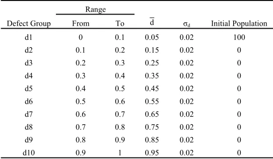
of which is presented here. For purpose of this study, it was chosen to divide the defect growth into 10 groups. This

value was chosen to correspond with the Federal Highways Agency inspection recommendations in the US, where

each element in a structure is assigned one of 10 of the National Bridge Inventory Condition Ratings [50]. The

possible range of defect sizes for each group is modelled statistically with an assumed mean and standard deviation,

as outlined in Table 1. The defect size is assumed to vary from 0-1.0, with a 0.1 defect range for each group (e.g.

crack width of a reinforced concrete structure varying from 0-1.0mm). The standard deviation of the groups

represents the scatter of the range of actual sizes of the defects in the group, and is not related to the error in sizing

of a defect. It was assumed that the standard deviation of the range of defect sizes in a group is independent of the

mean defect size of the group, and a constant value was assumed for each group. In addition, it was assumed initially

that there were 100 defects in the smallest defect group, and no defects in all other groups (i.e. taken to represent a

new structure), Table 1, although the methodology can consider a structure at any stage of its life.

Initially, for each value of ΔT, the two Markov matrices were used to calculate the stabilised number of defects in

each group (directly before inspection or failure), for each year in the ΔT cycle, for a given set of input parameters.

The methodology outlined was then used to determine the optimum time between inspections, and subsequently to

analyse the effect of the interaction of the quality of the inspection techniques for detection and sizing on the

optimum time between inspections and the expected annual total costs of the structure. The effect of the quality of

inspections on cost overrun, such as unnecessary repairs, was also investigated using the events based decision

theory described. This provides a powerful decision tool for infrastructure owners/managers in optimising

maintenance budget spend as based upon available funds, structural form, deterioration mechanism, environment

and limit state considered, it empowers them, rather than performing inspections on e.g. a bi-annual basis, using a

range of NDT tools to identify the best combination of techniques to be employed in assessing condition and

Accepted manuscript

5.1.

Optimal Time between Inspections

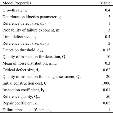
Table 2 shows the set of parameters assumed in the model for the purpose of this exercise. Using these parameters,

the optimum time between inspections was determined on the basis of the minimum expected annual total costs of

the structure, E

(

)

here that these are theoretical parameters selected to demonstrate the operability of the methodology. Research is

ongoing to identify realistic parameters to be employed based upon the NDT tool, deterioration mechanism, limit

state, cost etc [28, 29, 30, 31, 32, 33, 34]. Figure 11 shows the results of the analysis, illustrating that a period of

4-years represents the optimum inspection interval for the case considered.

As illustrated in Figure 11 the inspection interval has a significant effect on the expected annual total inspection

cost, E

(

)

(

)

from 60% of the total cost for a 1 year inspection interval, to just 10% of the total cost for a 10 year inspection

interval. As expected, an inverse trend emerges for the total failure cost, with the expected total failure cost ranging

from just 1.4% of the total cost at a 1 year inspection interval, to 48% of the total cost for a 10 year inspection

interval.

The expected total cost of repair, E

(

)

contributing to 58% of the total cost at the optimal inspection interval (ΔT=4). However, Figure 11 demonstrates

that the expected total cost of repair is relatively insensitive to the inspection interval. This is due to the

incorporation of the sizing assessment into the analysis, as the second stage of an inspection. Using this

methodology it is possible to determine the extent of each repair at the time of an inspection, and to estimate the cost

of repair based on the size of the defect, according to Equation 27. For example, if inspections are carried out

annually, then it is assumed that large defects are unlikely to develop, and only minor repairs are carried out every

year. Whereas if inspections are only carried out every 10 years, it is assumed that quite extensive repairs will be

necessary due to larger defects, but these repairs are less frequent. Therefore, there is just a 15% difference between

(

)

Accepted manuscript

5.2. Inspection

Quality

Using the methodology developed, it is possible to look at the interaction of the inspection methods for detection

and sizing, and see how this affects the optimum inspection interval and the expected annual total costs. This

provides the owner/manager with a useful decision tool when selecting a combination of inspection techniques to be

used as part of a maintenance management plan.

Figures 12-13 illustrate how a different combination of inspection techniques can affect the optimal maintenance

management plan, and the expected annual costs of the structure. In relation to the first inspection, a higher quality

technique, Q1, reduces the noise associated with the inspection procedure, and therefore, more accurately determines

which defects should be further assessed, which consequently reduces the number of failures due to undetected

defects. Figure 12 illustrates a direct relationship between the inspection quality for detection and the optimal

inspection interval. A similar trend emerges when the quality of the second technique, Q2, in increased. A better

technique reduces the number of failures, as a higher proportion of defects are sized correctly and repaired when

necessary.

The owner/manager has a number of options when using this new decision tool. In the case where a convenient

inspection interval has been decided upon, Figure 12 can be used to find a combination of technique qualities with

this inspection interval as optimal. Although this can result in a multiple of combinations of techniques, Figure 13

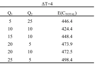
can then be used to determine which of these combinations results in the lowest expected annual costs. For example,

if an inspection interval of 4 years is convenient, from Figure 12, there are 6 different combinations of techniques

which would be suitable. These 6 combinations are listed in Table 3, with the expected annual total costs for each

combination, which are illustrated in Figure 13. In this case, the second option (Q1=10, Q2=10) results in the lowest

relative cost, and is clearly the most cost efficient combination of techniques for the chosen inspection interval of 4

years.

Alternatively, if the inspection for detection is chosen initially, Figures 12-13 can be used to choose a suitable

Accepted manuscript

possible to determine the optimal inspection interval, Figure 12, and the expected annual total costs of the structure,

Figure 13. Depending on the structure, it may be more convenient to carry out inspections less often (depending on

intangible costs/benefits that have not been incorporated into this model), even though the relative expected annual

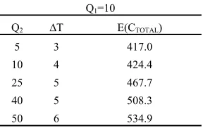
total cost is higher. Table 4 details a list of options available for a specific inspection quality for detection, Q1=10.

This method interestingly points out that there are two available options (for the quality of the second inspections)

that result in an optimal inspection interval of 5 years, yet one option has a relatively lower expected annual total

cost than the other, clearly showing it to be the most cost efficient choice. By looking at this interaction of

inspection techniques for detection and sizing assessment, an owner/manager can clearly pick the optimum

combination of techniques to suit a particular set of requirements.

Furthermore, using the events based decision theory outlined in Section 3, the effect of the quality of inspections on

cost overrun, such as unnecessary repair, can also be investigated. Figure 14 illustrates that the total cost of repair is

relatively insensitive to the quality of the second inspection, although it is clear that the inspection quality affects the

relative breakdown of these costs into necessary and unnecessary repairs. The number of repairs carried out

depends on the number of defects that are sized and are found to be greater than the critical defect size, therefore, the

cost overrun of unnecessary repairs reduces as more accurate inspections for sizing are carried out. By using a better

quality technique, the defects that could lead to failure of a component are repaired, rather than defects that are

incorrectly sized, and are not in need of repair. Reducing the number of failures within the structure has the effect of

increasing the optimal inspection interval. As discussed previously, although a higher inspection quality results in an

increase in the expected annual cost of a structure, Figure 13, the optimal inspection interval is likely to also

increase, Figure 12, which can be more convenient for an owner/manager of a structure.

6. Conclusions

This paper presents infrastructure owners/managers with a decision tool based upon the subdivision of the

Accepted manuscript

infrastructural elements/networks to minimise the probability of failure (i.e. limit state exceedance) within budgetary

constraints.

The paper demonstrates that the choice of inspection techniques for detection and sizing has a significant influence

on the optimum time between inspections, and hence the minimum annual total cost of the structure. When carrying

out an inspection there are two points of interest, the presence of a defect, and the size of a defect present. Since

each stage of the inspection has a different purpose, it is necessary to separate these procedures to accurately model

an inspection process which is to be incorporated into a maintenance management plan.

The separation of the inspection process into two stages enables the investigation to study the effect of both stages of

the inspection on the expected annual costs of the structure, and the maintenance plan for the structure. The

separation of these procedures and the interaction of the two inspection techniques have not previously been

considered.

By modelling the two stages of an inspection as separate procedures, using different parameters, the effect of

different combinations of techniques can be investigated. The detection process is similar to a screening exercise to

determine which defects require further assessment. By producing decision tools similar to Figures 12-13, it is

possible to look at the relative benefits of using different quality techniques. Depending on the requirements of the

owner/manager, upon the structure considered, its environment and deterioration mechanism, it may be more

convenient to use a low quality screening technique for detection and a higher quality inspection technique for sizing

to assess which defects should be repaired. The developed methodology allows for the first time, the effect of such

decisions to be evaluated quantitatively both with regard to performance (i.e. probability of limit state exceedance)

and budgetary cost (i.e. cost of assessment campaign and associated good/bad decisions). The combination of

techniques used during an inspection is demonstrated to effect the optimal time between inspections. If an inspection

requires partial or total closure of a structure, which can lead to user delays, the owner/manager may prefer to incur

a higher annual total cost in return for a longer optimal inspection interval. The results of each combination of

techniques can be assessed quantitatively with reference to Figures 12-13, allowing the most cost efficient approach

Accepted manuscript

Figures 12-13 demonstrates the benefits of the proposed approach. By modelling each stage of an inspection

separately, with different parameters, the interaction between these two inspection procedures and the effect of the

quality of the individual inspection methods on the optimal maintenance management plan and the annual costs of

the structure can be identified.

This methodology can be extended to spatial stochastic fields where inspections can be spatial dependent and the

sampling can be different for the kin of inspection. One way to solve this problem, is to base the description of the

defect and the error due to NDT on the polynomial chaos expansion [31].

Further work needs to be carried out on the calibration of parameters which were introduced as part of this model,

particularly in relating the parameters of the Weibull distribution (which are used to model the probability of failure)

to the actual mode of failure being considered (e.g. sudden or progressive failure) and investigating the most suitable

number of defect groups (and associated parameters) for the deterioration rate/mechanism being considered. Work is

also ongoing to further develop this method to enable the initiation stage of deterioration to be considered as well as

the propagation stage (which is particularly relevant for the deterioration of reinforced concrete due to chloride

ingress). Once this has been developed, it will also be possible to determine optimum repair materials, considering

the properties of the repair materials for both the initiation phase and propagation phase of deterioration.

Acknowledgements

The support of the European Union Interreg IIIb – Atlantic Area program through funding of the MEDACHS

research project (Project No. 197) is gratefully acknowledged.

Appendix A - Notation

CF = cost of failure for an individual defect

CI1 = cost of an individual inspection for detection

CI2 = cost of an individual inspection for sizing

Accepted manuscript

d = actual size of the defect

dc = critical defect size (a defect size greater than dc leads to a repair)

di = defect group i

d = mean defect size of a group

dmin = detection threshold

ref

d = reference defect size

ref_pf

d = reference defect size for the probability of failure, Weibull law parameter

d1 = limit defect size, Weibull law parameter

1

dˆ = size of the detected defect (from inspection 1)

2

dˆ = size of the defect from inspection (from inspection 2)

E( ) = annual expectancy of any cost variable

E1A = event 1 for sizing assessment – good sizing, no repair

E2A = event 2 for sizing assessment – wrong sizing, repair

E3A = event 3 for sizing assessment – wrong sizing, no repair

E4A = event 4 for sizing assessment – good sizing, repair

E1D = event 1 for detection – no defect, no detection

E2D = event 2 for detection – no defect, detection

E3D = event 3 for detection – defect, no detection

E4D = event 4 for detection – defect, detection

g = deterioration kinetics parameter

F

k = failure impact coefficient

I

k = inspection cost coefficient

R

k = repair cost coefficient

m = Weibull exponent (to calculatepf) which determines the spread of the curve

N = total number of groups

Accepted manuscript

PFA = probability of false alarm

PGANR = probability of a good assessment resulting in no repair

PGAR = probability of a good assessment resulting in repair

PoD = probability of detection

PWANR = probability of a wrong assessment resulting in no repair

PWAR = probability of a wrong assessment resulting in repair

f

p = annual probability of failure

ref

Q = reference inspection quality

Q1 = quality of the inspection method for defect detection

Q2 = quality of the inspection method for sizing assessment

ΔT = inspection interval in years

α = growth rate of a defect

σ

σ

σ

k

j@Y d

Accepted manuscript

References

[1] Enright, M.P. and Frangopol, D. M. (1999). “Maintenance planning for deteriorating concrete bridges.”

Journal of Structural Engineering, 125(12), 1407-1414

[2] Soltani, M. (1995). ‘‘Statistical bridge inspection.’’ Applications of statistics and probability, Lemaire, Favre,

and Mebarki, eds., Balkema,Rotterdam, The Netherlands, 387–391.

[3] Estes, A. C. and Frangopol, D. M. (1999). “Repair optimization of highway bridges using system reliability

approach.” Journal of Structural Engineering, 125(7), 766-775.

[4] Faber, M. H and Sorensen, J. D. (2002). “Indicators for inspection and maintenance planning of concrete

structures.” Journal of Structural Safety, 24(4), 377-396.

[5] Kong, J. S. and Frangopol, D. M. (2004). “Life cycle reliability-based maintenance cost optimisation of

deteriorating structures with emphasis on bridges” Journal of Structural Engineering, 129(6), 818-828.

[6] Kong, J. S. and Frangopol, D. M. (2004). “Cost-reliability interaction in life-cycle cost optimization of

deteriorating structures.” Journal of Structural Engineering, 130(11), 1704-1712.

[7] Kong, J. S. and Frangopol, D. M. (2005). “Probabilistic optimization of ageing structures considering

maintenance and failure costs.” Journal of Structural Engineering, 131(4), 600-616.

[8] Lauridsen, J., Bjerrum, J., Sloth, M. and Jensen, F. M. (2006). “Principles for a guideline for probability-based

management of deteriorated bridges.” IABMAS 2006 Conference, Bridge Maintenance, Safety and

Management (CD-Rom), Porto.

[9] O'Connor A. and Eichinger E., (2007), ‘Site-Specific Traffic Load Modelling for Bridge Assessment’, ICE

Journal of Bridge Engineering,160(4), 185 - 194.

[10] O'Connor A. and Enevoldsen I., (2009), ‘Probability based assessment of bridges according to the new Danish

guideline’, Structure and Infrastructure Engineering, 5(2), 157 - 168.

[11] O'Connor A. and O’Brien E., (2005), ‘Mathematical Traffic Load Modelling and Factors Influencing the

Accuracy of Predicted Extremes’, Canadian Journal of Civil Engineering, 32, pp. 270 - 278.

[12] Radojicic, A., Bailey, S. F. and Brühwiler, E. (2001). “Probabilistic models of cost for the management of

Accepted manuscript

[13] Stewart, M. G. (2001). “Reliability based assessment of ageing bridges using risk ranking and life cycle cost

decision analyses” Reliability Engineering and System Safety, 74(3), 263 – 273.

[14] Stewart, M. G., Estes, A. C. and Frangopol, D. M., (2004). “Bridge deck replacement for minimum expected

cost under multiple reliability constraints.” Journal of Structural Engineering, 130(9), 1414-1419.

[15] Stewart, M. G. (2005). “Life-cycle cost analysis considering spatial and temporal variability of

corrosion-induced damage and repair of concrete surfaces.” International Conference on Structural Safety and

Reliability, ICOSSAR, Rome, Italy.

[16] Stewart, M. G. and Mullard, J. A. (2006). “Reliability based assessment of the influence of concrete durability

on the timing of repair for RC bridges.” IABMAS 2006 Conference, Bridge Maintenance, Safety and

Management (CD-Rom), Porto.

[17] Corotis, R.B., Ellis J.H. and Jiang, M. (2005). “Modelling of risk-based inspection, maintenance and life-cycle

cost with partially observable Markov decision processes.” Structure and Infrastructure Engineering, 1(1),

75-84.

[18] Schoefs, F. and Clement, A. (2004). “Multiple inspection modeling for decision making and management of

jacket offshore platforms: effect of false alarms.” International Forum on Engineering Decision Making,

IFED, Stoos,Switzerland.

[19] Rouhan, A. and Schoefs, F. (2003). “Probabilistic modeling of inspection results for offshore structures”.

Journal of Structural Safety, 25(4), 379-399.

[20] Straub, D, and Faber, M.H. (2003). “Modeling dependency in inspection performance.” Applications of

Statistics and Probability in Civil Engineering, Rotterdam, 1123-1130.

[21] Chung, H. Y., Manuel, L. and Frank, K. H. (2006). “Optimal inspection scheduling of steel bridges using

nondestructive testing techniques.” Journal of Bridge Engineering, 11(3), 305-319.

[22] Zhang, R. and Mahadevan, S. (2001). “Fatigue reliability using nondestructive inspection.” Journal of

Structural Engineering, 127(8), 957-965

[23] James, L.A. (1997). “Surface-crack aspect ratio development during corrosion-fatigue crack growth in low

Accepted manuscript

[24] Pellerin, R.F, Lavinder, J.A., Ross, R.J. and Falk, R.H. (1996). ”Non destructive evaluation of timber bridges.”

Proceedings of SPIE – The International Society for Optical Engineering: Non destructive evaluation of

materials and composites, 2994, 275 – 284.

[25] DNV 2007, Statistical representation of soil data, Recommended practice DNV-RP-C207, Det Norske Veritas,

April 2007.

[26] Madsen, H., Skjong, R., Tallin, A. and Kirkemo, F. (1987). “Probabilistic fatigue crack growth analysis of

offshore structures, with reliability updating through inspection.” Marine Structural Reliability Symposium,

Arlington, Virginia, 45-55.

[27] Onoufriou, T. and Frangopol D. M. (2002). “Reliability-based inspection optimisation of complex structures: a

brief retrospective.” Journal of Computers and Structures, 80(12), 1133-1144.

[28] Barnouin, B., Lemoine, L, Dover, W.D., Rudlin, J., Fabbri, S., Rebourcet, G., Topp, D., Kare, R., Sangouard,

D. (1993). “Underwater inspection reliability trials for offshore structures”. In ASME NY, editor. Proc. of the

12th OMAE conference. Vol. 2 pp. 883-890.

[29] Bonnet, S., Schoefs, F., Ricardo, J., Salta, M.M. (2008). “Statistical study and probabilistic modelling of error

when building chloride profiles”, Proceeding of 1st International Conference on Applications Heritage and

Constructions in Coastal and Marine Environment, (MEDACHS’08), paper #111, 8 pages, 28-30 January

2008, Lisbon (LNEC), Portugal (2008).

[30] Bonnet, S., Schoefs, F., Ricardo, J., Salta, M. (2009). “Statistical study and probabilistic modelling of error

when building chloride profiles for reliability assessment”, to appear in Material and Structures, 2009

[31] Schoefs, F. (2008). “Risk analysis of structures in presence of stochastic fields of deterioration: coupling of

inspection and structural reliability”, to appear in Australian Journal of Structural Engineering, Special

“Engineering Decision Making issue” Issue, guest editors Mark Stewart and Stuart Reid.

[32] Schoefs, F., Clément, A., Nouy, A. (2009) ‘‘Assessment of spatially dependent ROC curves for inspection of

random fields of defects”, to appear in Structural Safety,Ed. 2009

[33] Pakrashi, V., Schoefs, F., Memet, J.B., O’Connor, A. (2008) “An Image Analysis Based Damage Classification

Accepted manuscript

[34] Boéro, J., Schoefs, F., Capra, B. (2008). “Expert Judgement for Combining NDT Tools in RBI context:

Application to Marine Structures”, Proc. of 4th International ASRANet Colloquium, 25–27 June 2008, Athens,

Greece, paper 70, 9 pages, proc. on CD-Rom.

[35] Breysse, D., Schoefs, F., Salta, M. and Bonnet, S. (2007) “Assessment updating of corrosion accounting

uncertainties in modelling and NDT measurements.” ICASP10 2007 conference, Tokyo.

[36] Scherer, W.T. and Glagola, D.M. (1994). “Markovian models for bridge maintenance management.” Journal of

Transportation Engineering, 120(1), 37-51.

[37] Ang, A. H-S. and Tang, W. N. (1975) Probability Concepts in Engineering Planning and Design Volume I,

Basic Principles. John Wiley and Sons, New York.

[38] Roelfstra, G., Hajdin, R., Adey, B. and Brühwiler, E. (2004). “Condition Evolution in Bridge Management

Systems and Corrosion-Induced Deterioration”. Journal of Bridge Engineering, 9(3), 268-277.

[39] Orcesi, A., and Crémona, C. (2006). “Optimisation de la gestion des ponts en béton armé par chaînes de

Markov (In French)”, “Optimized management of reinforced concrete bridges using Markov chains”. Bulletin

des Laboratoires des Ponts et Chausées, 265, 19-33.

[40] Micevski, T., Kuczera, G. and Coombes, P. (2002). “Markov model for storm water pipe deterioration.”

Journal of Infrastructure Systems, 8(2), 48-56.

[41] Poinard, D., Le Gauffre, P. and Haidar (2003). “Markov model and climate factors for the rehabilitation

planning of water networks.” Proc. 17th _{European Junior Scientist Workshop Rehabilitation Management of}

Urban Infrastructure Networks, Neunzehnhain, Germany, September 2003.

[42] Mori, Y. and Ellingwood, B.R. (1994b). “Maintaining reliability of concrete structures. II: Optimum

inspection/repair.” Journal of Structural Engineering, 120(3), 846-862.

[43] Straub, D. and Faber, M.H. (2005). “Risk based inspection planning for structural systems.” Structural Safety,

27(4), 335-355.

[44] Straub, D. and Faber, M.H. (2004). “System effects in generic risk-based inspection planning.” Journal of

Offshore Mechanics and Arctic Engineering, 126(3), 265-271.

[45] Adey, B., Bernard, O. and Gérard, B. (2003). “Risk-based replacement strategies for deteriorating reinforced concrete pipes.” Proceedings of 2nd International RILEM Workshop on Life Prediction and Aging

Accepted manuscript

[46] Kong, J.S. and Frangopol, D.M. (2003). “Life-cycle reliability-based maintenance cost optimisation of

deteriorating structures with emphasis on bridges.” Journal of Structural Engineering, 129(6), 818-828.

[47] Weibull, W. (1951). “A statistical distribution function of wide applicability.” Journal of Applied Mechanics,

18(3), 293-297.

[48] Ang, A. H-S. and Tang, W. N. (1984) Probability Concepts in Engineering Planning and Design Volume II,

Decision Risk and Reliability. John Wiley and Sons, New York.

[49] Bonnet S., Schoefs F., Ricardo J., Salta M. (2009), “Effect of Error Measurement of Chloride Profiles on

Reliability Assessment”, H. Furuta, D.M. Frangopol & M. Shinozuka (eds), ICOSSAR’09, Osaka, Japan,

September 13-19,2009.

[50] Estes, A.C. and Frangopol, D.M. (2001). “Bridge lifetime system reliability under multiple limit states.”

Journal of Bridge Engineering, 6(6), 523-528.

Accepted manuscript

Table Captions

Table 1. Defect group data used in the model

Table 2. Parameter values used in Markov Maintenance model Table 3. Inspection technique combination 1

Accepted manuscript

Range

Defect Group From To d σd Initial Population

d1 0 0.1 0.05 0.02 100

d2 0.1 0.2 0.15 0.02 0

d3 0.2 0.3 0.25 0.02 0

d4 0.3 0.4 0.35 0.02 0

d5 0.4 0.5 0.45 0.02 0

d6 0.5 0.6 0.55 0.02 0

d7 0.6 0.7 0.65 0.02 0

d8 0.7 0.8 0.75 0.02 0

d9 0.8 0.9 0.85 0.02 0

Accepted manuscript

Model Properties Value

Growth rate, α 0.4

Deterioration kinetics parameter, g 3

Reference defect size, dref 1

Probability of failure e