Streamflow Decomposition Based Integrated ANN Model
Nikhil Bhatia, Laksha Sharma, Shreya Srivastava, Nidhish Katyal, Roshan Srivastav
School of Mechanical and Building Sciences, VIT University, Vellore, India. Email: [email protected]
Received October 10th, 2012; revised November 17th, 2012; accepted November 29th, 2012
ABSTRACT
The prediction of riverflows requires the understanding of rainfall-runoff process which is highly nonlinear, dynamic and complex in nature. In this research streamflow decomposition based integrated ANN (SD-ANN) model is devel- oped to improve the efficacy rather than using a single ANN model for the flow hydrograph. The streamflows are de- composed into two states namely 1) the rise state and 2) the fall state. The rainfall-runoff data obtained from the Kolar River basin is used to test the efficacy of the proposed model when compared to feed-forward ANN model (FF-ANN). The results obtained in this study indicate that the proposed SD-ANN model outperforms the single ANN model in terms of both the statistical indices and the prediction of high flows.
Keywords: Artificial Neural Network; Rainfall-Runoff Modeling; Streamflow Decomposing; Black Box Modelling
1. Introduction
A wide variety of rainfall-runoff models have been de- veloped and applied for water resources planning which is vital in terms of flood control and management. Tradi- tionally, the hydrologists and water resources researchers have used conventional modeling techniques either de- terministic models that includes physics of the underly- ing process or systems theoretic (black box) models. However these models require a large quantity of data and a complex methodology for its calibration. Most of the hydrological models either show unsuccessful results or become cumbersome. Many researchers report that these models fail to capture the high flows in a hydro- graph [1,2] due to limited data sets available in the high flow domain (5% of total calibrating patterns) for cap- turing the nonlinear dynamics.
Recently the researchers have focused to decompose the data corresponding to flow hydrograph to enhance the performance of the hydrologic models. Mostly the studies have concentrated on using either the statistical techniques or soft decomposing techniques for data de- composition [3]. Studies include automated base flow separation and recession analysis [4], spectral analysis [5], wavelet transforms and runoff time series analysis [6-9], modular neural network (MNN) [10], self-orga- nizing map (SOM) classifier [11,12] and self organizing linear output map (SOLO) [13]. Most of these studies conclude that the decomposition and partitioning of data resulted in better model performance.
Artificial neural network (ANN) has been proposed by
researchers which is a system theoretic model that has gained momentum in the last few decades as it has been successfully applied to a wide range of problems in hy- drology [2,14-16]. It is used to develop relationship be- tween input and output variables using the existing data. Jain and Srinivasulu [3] proposed an integrated approach to model decomposed flow hydrograph using ANN and conceptual techniques. The streamflow decomposition was carried out based on physical processes which divide the input-output and fit the models for each of the seg- ments [3]. However, the models developed using the distributed approach would have made the solution pro- cedures complex significantly [3]. In this study, efforts are made to develop a simplified ANN based decom- posed streamflow model without requiring any prior knowledge or understanding of physical processes. In this study the data is divided into two states namely rise and fall, based on the current state. The proposed model is compared with the feed forward ANN model, on a real case example of Kolar basin, India.
This paper is organized as follows. Section 2 provides a brief introduction on ANN. Section 3 describes pro- posed methodology. Section 4 illustrates the case study on Kolar basin, India. Section 5 includes Results and Discussion and the paper is concluded with summary and conclusions presented in Section 6.
2. Artificial Neural Network
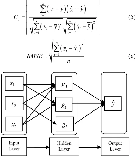
It attempts to develop the massively parallel local proc- essing and the distributed storage properties which are believed to exist in the human brain [17]. Simple proc- essing units of an ANN are called “neurons”. Neurons having similar characteristics are grouped in one single layer (neurons in an input layer receive an input from the external source, and transmit the same to a neuron in an adjacent layer, which could either be a hidden layer or an output layer). Structure of the ANN Model is shown in
Figure 1.
The general mathematical form of an ANN Model is given as:
1
ˆ i n i i
i
y f V u x W
(1) where, xi is the input of the ANN Model, i is the
weight connecting input nodes to hidden nodes, Vi is
the weight connecting hidden nodes to output nodes, W
,
are the bias at hidden and output layer respectively
and are the activation functions at hidden
and output layer respectively.
,u f
The weights Wi and Vi are usually determined by
minimizing the quadratic error function,
21 ˆ
2
E y
n
y
(2)Once the ANN Model is executed then the error at the output layer from an ANN can be computed if output is known.
ˆ y y
(3) where, is the error at the output layer, y is the
ob-served stream flow and y is the estimated stream flow.
Using the process of the feed-forward calculations and back-propagation of the errors the connection strengths are updated and an acceptable level of output is predicted. This is called as training of an ANN. Once the network has been trained, it can be tested using the testing data.
3. Model Development
Determination of significant input variables is a very essential step in ANN Modeling [18,19]. Cross correla- tion is used to find the relationship between the variables [2,19-21] and is used to represent the most popular ana- lytical techniques for selecting appropriate inputs [18]. Observed relationships between the training samples and the connection weights enhance generalization ability of an ANN model [22].
The inputs to the SD-ANN model were selected on the basis of cross- and auto-correlation method as proposed by Sudheer et al. [2]. The significant input variables were
found to be the effective rainfalls at lag time steps of t −
9, t − 8, and t − 7 ( 9 8 an d t 7) using the cross-
correlation and the river flow values at lag time steps of t
− 1 and t − 2 ( t 1
, t t
P P P
Q and Qt2) using the autocorrelation function [23]. The output of the model is the riverflow at time t (Qt). Thus Qt is represented as
P9,Pt8,Pt7,Qt1,Qt2
t t
Q f (4)
In this study, the hourly input data are divided into two cases based on the previous data sets,
1) Rise: In the rise pattern the value of runoff at time t
is greater than that of time step t − 1, i.e., Qt Qt1.
2) Fall: In the fall pattern the value of runoff at time t
[image:2.595.313.533.622.709.2]− 1 is greater than that of time step t, i.e., t1 t. Figure 2 shows the proposed methodology in which
Model 1 decomposes the data into classes (i.e., rise and
fall) based on the input variables, Model 2 is the cali- brated ANN, model for the rise and Model 3 is the cali- brated ANN model for the fall.
Q Q
Statistical indices like the coefficient of correlation (Cc), root-mean-square error (RMSE) and Nash-Sutcliffe
efficiency (NSE) [24] are used to evaluate the perform-
ance of the model. The equations of these statistical in- dices are,
1 n i 2 2 1 1 ˆ ˆ ˆ ˆ i i n n i i i iy y y y
y y y y
c C
(5)
21 ˆ n i i i y y n
RMSE (6)
x1 2 x 3
x
1 g 2g
3g
ˆ
y
Input Layer Hidden Layer Output LayerFigure 1. Typical model structure of the FF-ANN model.
Input Model 1
Model 2 Model 3 Rise Fal Output l
2
1
2
1
ˆ 1
n
i i i
n
i i
y y NSE
y y
(7)where i is the Observed Runoff Value, i is the Pre-
dicted Runoff Value, y is the mean of the observed run-
off values and
y y
ˆ
yis the mean of the predicted runoff values.
4. Case Study
A case study on the Kolar River basin is chosen to dem- onstrate the proposed SD-ANN method. FF-ANN and SD-ANN models for forecasting the runoff values at 1-hour lead time have been developed. Data relating to monsoon season (i.e., July, August, and September) for 3
years period (from 1987 to 1989). Note that areal average values of rainfall data for three rain gauge stations were used in the study.
The Kolar River is a tributary of the river Narmada that drains an area about 1350 km2 before its confluence
with Narmada near Neelkant (Figure 3). In this study the
catchment area up to the Satrana gauging site is consid-ered, which constitutes an area of 903.87 km2. The
75.3-km-long river course lies between north latitude
and east longitude Further
more details on the basin are given by Nayak et al. [25].
21 09 ' - 23 17 ' 77 01' - 77 29 '
From the total available data for 3 years, 6525 patterns (input-output pairs) were identified for the study and were split into calibration (5500 sets, 1987-1988 data sets) and validation (1025 sets, 1989 data sets). Note that the 1025 sets considered for validation were corresponding to a continuous hydrograph.
[image:3.595.107.199.88.136.2]The activation function used at the hidden layer and at the output layer is sigmoid function as it is easily differ- entiable.
Figure 3. Map of Kolar river basin [25].
1
1 x
y
e
(8) To calculate the network parameters back propagation algorithm [26] has been used. Adaptive learning and momentum rates have been employed for the model training [25].
5. Results and Discussions
As discussed earlier, the SD-ANN model developed is used for forecasting the river flow for Kolar Basin at a lead time of 1 hour. The performance of the proposed SD-ANN model and FF-ANN model have been evalu- ated by means of a variety of statistical criteriasuch as coefficient of correlation (CC), coefficient of efficiency
(NSE) and the root-mean-square error (RMSE) between
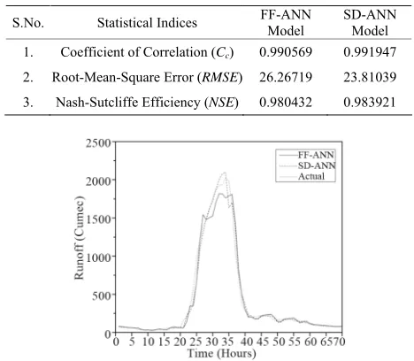
the actual and estimated flowvalues. The various statis- tics stated below in Table 1 indicates that the predicted
[image:3.595.305.539.506.710.2]value of runoff by the SD-ANN is more accurate than that of FF-ANN Model. Performance of both the models in terms of statistical indices is very similar and satisfac- tory as the correlation coefficient of both the models are very close to the unity. Further it is observed from the
Table 1 that the efficiency of both the models is greater
than 90% which is highly satisfactory according to Sham- seldin [27]. In addition, it is worth noting that the RMSE of the proposed model is less when compared to the FF-ANN model. Also the prediction of high flows is well modeled by the proposed SD-ANN model when com- pared to the FF-ANN model (Figure 4). It is evident
from the results that the decomposition of the streamflow has considerable impact on the performance of models.
Table 1. Statistical indices—comparison between SD-ANN and FF-ANN model.
S.No. Statistical Indices FF-ANN Model SD-ANN Model
1. Coefficient of Correlation (Cc) 0.990569 0.991947
2. Root-Mean-Square Error (RMSE) 26.26719 23.81039 3. Nash-Sutcliffe Efficiency (NSE) 0.980432 0.983921
[image:3.595.68.276.530.719.2]6. Summary and Conclusion
In this study, a simplified ANN based decomposed streamflow model is developed. The proposed data de- composition does not require any prior knowledge or understanding of physical processes. In this study the data is divided into two states namely rise and fall, based on the current state. The performance of the proposed SD-ANN model is compared to that of the feed-forward ANN model in terms of statistical indices such as coeffi- cient of correlation, coefficient of efficiency and root means square error. The exercise was carried out for the hourly data in Kolar river basin, India. It is observed that the proposed SD-ANN model and the FF-ANN model show similar results in terms of statistical indices except the case of RMSE where the former outperforms the
lat-ter. Further, the SD-ANN model outperforms the FF- ANN model in prediction of high flows. The results show the significance of the streamflow decomposition when compared to single hydrograph. The performance of the SD-ANN models has to be tested on various time scales. Further extensions of this model can be examined to improve the forecasting accuracy [28].
7. Acknowledgements
The authors thank the Vellore Institute of Technology, Vellore, India, for providing the necessary facilities to carry out this research work.
REFERENCES
[1] C. E. Imrie, S. Durucan and A. Korre, “River Flow Pre- diction Using Artificial Neural Networks: Generalization beyond the Calibration Range,” Journal of Hydrology,
Vol. 233, No. 1-4, 2000, pp. 138-153. doi:10.1016/S0022-1694(00)00228-6
[2] K. P. Sudheer, A. K. Gosain and K. S. Ramasastri, “A Data-Driven Algorithm for Constructing Artificial Neural Network Rainfall-Runoff Models,” Hydrological Proc- esses, Vol. 16, No. 6, 2002, pp. 1325-1330.
doi:10.1002/hyp.554
[3] A. Jain and S. Srinivasulu, “Integrated Approach to Mo- del Decomposed Flow Hydrograph Using Artificial Neu- ral Network and Conceptual Techniques,” Journal of Hy- drology, Vol. 317, No. 3-4, 2005, pp. 291-306.
[4] J. G. Arnold, P. M. Allen, R. Muttiah and G. Bernhardt, “Automated Base Flow Separation and Recession Analy- sis Techniques,” Ground Water, Vol. 33, No. 6, 1995, pp. 1010-1018. doi:10.1111/j.1745-6584.1995.tb00046.x [5] M. E. Spongberg, “Spectral Analysis of Base Flow Sepa-
ration with Digital Filters,” Water Resources Research, Vol. 36, No. 3, 2000, pp. 745-752.
doi:10.1029/1999WR900303
[6] L. C. Smith, D. L. Turcotte and B. L. Isacks, “Streamflow Characterization and Feature Detection Using a Discrete Wavelet Transform,” Hydrological Processes, Vol. 12, No.
2, 1998, pp. 233-249.
doi:10.1002/(SICI)1099-1085(199802)12:2<233::AID-H YP573>3.0.CO;2-3
[7] D. Labat, R. Ababou and A. Mangin, “Rainfall-Runoff Relations for Karstic Springs. Part II: Continuous Wave- let and Discrete Orthogonal Multiresolution,” Journal of Hydrology, Vol. 238, No. 3-4, 2000, pp. 149-178.
doi:10.1016/S0022-1694(00)00322-X
[8] S. Y. Liu, X. Z. Quan and Y. C. Zhang, “Application of Wavelet Transform in Runoff Sequence Analysis,” Pro- gress in Nature Science, Vol. 13, No. 7, 2003, pp. 546-
549.
[9] F. Anctil and D. G. Tape, “An Exploration of Artificial Neural Network Rainfall-Runoff Forecasting Combined with Wavelet Decomposition,” Journal of Environmental Engineering and Science, Vol. 3, No. 1, 2004, pp. S121-
S128. doi:10.1139/s03-071
[10] B. Zhang and S. Govindaraju, “Prediction of Watershed Runoff Using Bayesian Concepts and Modular Neural Networks,” Water Resources Research, Vol. 36, No. 3, 2000, pp. 753-762. doi:10.1029/1999WR900264
[11] D. Furundzic, “Application Example of Neural Networks for Time Series Analysis: Rainfall Runoff Modeling,”
Signal Processing, Vol. 64, No. 3, 1998, pp. 383-396.
doi:10.1016/S0165-1684(97)00203-X
[12] R. J. Abrahart and L. See, “Comparing Neural Network and Autoregressive Moving Average Techniques for the Provision of Continuous River Flow Forecasts in Two Contrasting Catchments,” Hydrological Processes, Vol.
14, No. 11-12, 2000, pp. 2157-2172.
doi:10.1002/1099-1085(20000815/30)14:11/12<2157::AI D-HYP57>3.0.CO;2-S
[13] K. L. Hsu, H. V. Gupta, X. Gao, S. Sorooshian and B. Imam, “Self-Organizing Linear Output Map (SOLO): An Artificial Neural Network Suitable for Hydrologic Mod- eling and Analysis,” Water Resources Research, Vol. 38,
No. 12, 2002, pp. 1-17. doi:10.1029/2001WR000795 [14] K. Hsu, V. H. Gupta and S. Sorooshian, “Artificial Neural
Network Modeling of the Rainfall-Runoff Process,” Wa- ter Resources Research, Vol. 31, No. 10, 1995, pp. 2517- 2530. doi:10.1029/95WR01955
[15] N. Sajikumar and B. S. Thandaveswara, “A Nonlinear Rainfall-Runoff Model Using an Artificial Neural Net- work,” Journal of Hydrology, Vol. 216, No. 1-2, 1999, pp.
32-55.
[16] K. P. Sudheer, P. C. Nayak and K. S. Ramasastri, “Im- proving Peak Flow Estimates in Artificial Neural Net- work River Flow Models,” Hydrological Processes, Vol.
17, No. 3, 2003, pp. 677-686. doi:10.1002/hyp.5103 [17] M. J. Zurada, “An Introduction to Artificial Neural
Sys-tems,” West Publishing Company, St Paul, 1997. [18] G. J. Bowden, G. C. Dandy and H. R. Maier, “Input De-
termination for Neural Network Models in Water Re- sources Applications: 1. Background and Methodology,”
Journal of Hydrology, Vol. 301, No. 1-4, 2004, pp. 75-92.
Journal of Hydrology, Vol. 301, No. 1-4, 2004, pp. 93-
107.
[20] K. C. Luk, J. E. Ball and A. Sharma, “A Study of Optimal Model Lag and Spatial Inputs to Artificial Neural Net- work for Rainfall Forecasting,” Journal of Hydrology,
Vol. 227, No. 1-4, 2000, pp. 56-65. doi:10.1016/S0022-1694(99)00165-1
[21] D. Silverman and J. A. Dracup, “Artificial Neural Net- works and Long-Range Precipitation Prediction in Cali- fornia,” Journal of Climate and Applied Meteorology, Vol. 39, No. 1, 2000, pp. 57-66.
doi:10.1175/1520-0450(2000)039<0057:ANNALR>2.0.C O;2
[22] H. R. Maier and G. C. Dandy, “Neural Networks for the Prediction and Forecasting of Water Resources Variables: A Review of Modeling Issues and Applications,” Envi- ronmental Modelling & Software, Vol. 15, No. 1, 2000, pp. 101-124. doi:10.1016/S1364-8152(99)00007-9 [23] R. K. Srivastav, K. P. Sudheer and I. Chaubey, “A Sim-
plified Approach to Quantifying Predictive and Paramet- ric Uncertainty in Artificial Neural Network Hydrologic Models,” Water Resources Research, Vol. 43, No. 10, 2007, Article ID: W10407. doi:10.1029/2006WR005352
[24] J. E. Nash and J. V. Sutcliffe, “River Flow Forecasting through Conceptual Models: 1. A Discussion of Princi- ples,” Journal of Hydrology, Vol. 10, No. 3, 1970, pp.
282-290. doi:10.1016/0022-1694(70)90255-6
[25] P. C. Nayak, K. P. Sudheer, D. M. Rangan and K. S. Ramasastri, “Short-Term Flood Forecasting with a Neu- rofuzzy Model,” Water Resources Research, Vol. 41, No.
4, 2005, Article ID: W04004. doi:10.1029/2004WR003562
[26] D. E. Rumelhart, G. E. Hinton and R. J. Williams, “Learn- ing Representations by Back-Propagating Errors,” Nature,
Vol. 323, No. 6088, 1986, pp. 533-536. doi:10.1038/323533a0
[27] A. Y. Shamseldin, “Application of a Neural Network Te- chnique to Rainfall-Runoff Modelling,” Journal of Hy- drology, Vol. 199, No. 3-4, 1997, pp. 272-294.
doi:10.1016/S0022-1694(96)03330-6
[28] P. Mittal, S. Chowdhury, S. Roy, N. Bhatia and R. Sri- vastav, “Dual Artificial Neural Network for Rainfall-Run- off Forecasting,” Journal of Water Resource and Protec- tion, Vol. 4, No. 12, 2012, pp. 1024-1028.