Noise Source Location in Turbomachinery Using Coherence Based Modal Decomposition (AIAA 2009 3367)

Noise Source Location in Turbomachinery Using

Coherence Based Modal Decomposition

Gareth J. Bennett

,

Ciaran O’Reilly

Ulf Tapken

German Aerospace Center (DLR), Institute of Propulsion Technology, Engine Acoustics Branch

John Fitzpatrick

Coherence based source analysis techniques can be used to identify the contribution of turbomachinery core noise sources to pressure measurements in the far-field. The usual approach is to locate a measurement sensor within the engine and to calculate the ordinary coherence function between this and the far-field pressure measurement. If the internal measurement is close to a dominant noise source, the technique will identify this sources’ contribution to the overall far-field energy. Modal decomposition is an advanced technique which can provide detailed information as to the modal content of sound propagating in ducts. When applied to aero-engines, the technique can be used as a diagnostic to determine which of the many rotor-stator stages contribute most to the overall radiated sound power. The method developed in this paper discusses how the two techniques can be combined to locate the plane at which a mode is generated within an aeroengine. A proof of concept of the technique is successfully demonstrated with the use of simulated data.

I.

Introduction

Coherence-based noise source identification techniques can be used to identify the contribution of core noise to near and far field acoustic measurements of aero-engines. Karchmer and Reshotko1, 2_{and Reshotko}

and Karchmer3 _{used the ordinary coherence function between internal measurements and farfield}

micro-phones and derived the core noise at farfield locations by calculating the coherent output power (COP): a technique reported initially by Halvorsen and Bendat4_{. Karchmer}5 _{also used the conditioned coherency}

function to determine where the source region for core noise was located. Extraneous noise contamination at an internal microphone location can result in the derived core noise at the farfield location being signif-icantly lower than the true value. For such situations, Shivashankara6, 7 used Chung’s8 flow noise rejection technique, to identify the internal core noise contribution to farfield noise measurements. Hsu and Ahuja9

extended Chung’s technique to develop a partial-coherence based technique, that uses five microphones, to extract ejector internal mixing noise from farfield signatures which were assumed to contain the ejector mix-ing noise, the externally generated mixmix-ing noise, and also another correlated mixmix-ing noise presumably from the ejector inlet. Wherever there is more than one source, all of these approaches necessitate the location of at least one sensor near one of the sources, e.g. the core noise source, in order to measure that source in isolation. Where there is only one source in the presence of extraneous noise, it has been shown when using Chung’s technique, that no direct measure of the source is necessary. Minami and Ahuja10 _{discuss a}

technique where only farfield measurements are needed to separate any number of correlated sources from extraneous noise, which due to its distributed nature, could be jet noise for example. Previously published

∗_{Lecturer, Dept. of Mechanical and Manufacturing Engineering, Trinity College, Dublin 2, Ireland. AIAA Member.} †_{Research Fellow, Dept. of Mechanical and Manufacturing Engineering, Trinity College, Dublin 2, Ireland.} ‡_{Research assistant, Mller-Breslau-Str. 8, 10623 Berlin, Germany.}

work in this area from the 1970’s and 1980’s has been revisited in more recent years by Hsu and Ahuja9

and Nance.11 _{In Bennett and Fitzpatrick,}12 _{techniques which can be used to identify the contribution of}

combustion noise to near and far-field acoustic measurements of aero-engines were evaluated. When the core noise propagates in a non-linear fashion the identified contribution using ordinary coherence methods will be inaccurate. In the paper by Bennett and Fitzpatrick,13 _{an analysis technique to enable the contribution}

of linear and non-linear mechanisms to the propagated sound to be identified was reported. The technique was then applied to data from a small scale rig and to data from full scale turbo-fan engine tests. These techniques using tonal interactions were extended to examine bandlimited noise in the paper by Bennettet al.14

The sound fields in the inlet and outlet ducts of axial fans, compressors and aircraft engines propagate as higher order spinning acoustical modes in a wide frequency range. An in-duct modal decomposition technique is a measurement procedure from which one can determine the amplitudes of the acoustic modes propagating in a duct. A number of techniques have been reported which employ different methods to measure these modes for tonal and broadband noise sources15–20_{. Those techniques which decompose the}

sound field into incident and reflected radial modes using flush mounted microphones, in particular those of Yardley,21 _˚Abom22 _{and Enghardtet al,}15_{are of interest here.}

II.

Acoustic Pressure Field in a Cylindrical Duct

The usual approach in the analysis of duct acoustics is to approximate the duct by an infinite cylinder and to solve the differential equations by separation of variables. This leads to an eigenvalue problem, the solution of which gives the duct propagation modes. Each mode represents a different way in which sound may travel down the duct. A complete description of the sound field in the duct consists of knowing the complex amplitude of each mode.

A. Description of Mode Propagation in Hard Walled Cylindrical Flow Ducts

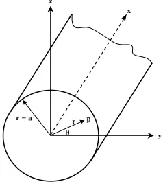
For acoustic propagation in an infinite hard walled cylindrical duct with superimposed constant mean flow velocity −→V, the pressure, p = p(r, θ, x, t), in cylindrical coordinates as defined by figure 1, is found as a solution of the homogeneous convective wave equation,

Figure 1. Polar coordinate system for a cylindrical duct, (r, θ, x)

1

c2

D2_p

Dt2 −

∂2_p

∂x2 −

1

r ∂ ∂r

r∂p ∂r

− 1

r2

∂2_p

∂θ2 = 0 (1)

where the substantive derivative is defined to be

D Dt =

∂ ∂t+

− →

V ∂ ∂x

This solution is found as a combination of the characteristic functions of equation (1) each of which satisfy specific boundary conditions. Rigorous treatments of the derivation of the separation-of-variables solution can be found in the literature23–25_.

For the following assumptions

2 of 18

• The flow is incompressible medium and isentropic with negligible temperature gradients.

• The mean flow speed,U= (Ux,0,0) is stationary with time.

• The axial mean flow profile as well as the duct scross-sectional area are invarient in the axial direction.

• The mean temperature and the density are stationary in space and time.

the solution to the wave equation for complex pressure can be given by a linear superposition of modal terms:

ˆ

p(x, r, ϕ) =

∞

X

m=−∞

∞

X

n=0

h

A+_m,ne(−jk+m,nx)+A−

m,ne

(+jk−m,nx)

i

fm,n(r)e(jmϕ) (2)

whereA+

m,nandA

−

m,nare the complex amplitudes of the modes,k+m,nxandk

−

m,nxare the axial wave numbers,

andmandnare the azimuthal and radial mode indices respectively. The + superscript refers to the direction of flow whereas the−superscript indicates the parameter to be defined counter to the flow direction. In the case of hard-walled acoustic boundary conditions, the modes form an orthogonal eigensystem, with a modal shape factor given by

fm,n(r) =

Jm(σmnr/R)

p

Nm,n

(3)

for a non-annular cylinder. In equation (3), Jmis a Bessel function of the first kind of ordermwith associated

hard-walled cylindrical eigenvalueσmn. R is the duct outer radius and in order to satisfy orthogonality the

normalisation factor is calculated to be

Nmn= 2π

Z R

0

J2_m(σmnr/R)r dr=πR2 J2m(σmn)−Jm−1(σmn) Jm+1(σmn) (4)

The normalisation transforms the orthogonal mode eigensystem into an orthonormal mode eigensystem. A mean flow is accommodated for in the formulation by modification of the axial wave numbers which is a function of the mode eigenvalue σmn and the free field propagation wave number, k, and is defined as

follows

k±

mn=k

−Mx±αmn

β2 (5)

where

αmn=

s

1− _βσ

mn

kR

2

(6)

and

β=p1−M2

x (7)

III.

Acoustic Modal Decomposition in Hard Walled Annular Flow Ducts

A. Introduction

The method employed in this paper is based on the approach proposed by ˚Abom.22 _Bennett,26 _who

imple-mented this technique with experimental data, decomposed the pressure field in such a way as to have the following characteristics:

• Incident and reflected modes can be identified;

• A mean flow can be accommodated;

• Radial, as well as azimuthal, modes can be identified;

• Duct-wall flush-mounted microphones only are used for the decomposition;

• The decomposition is performed for all frequencies not only at the BPF and harmonics;

• Data is acquired at all measurement locations simultaneously.

The procedure uses an array of axially and azimuthally distributed flush mounted microphones, and consists of solving equation (2) for the modal amplitudes,A±

m,n.

B. Mathematical Formulation of Modal Decomposition Technique

Another common way of expressing equation (2), as used by Enghardt et al15 _{and Tapken et al,}27 _and

one where the functional form of Am,n is expressed explicitly, is where the complex circumferential mode

distribution is isolated, being a function ofϕonly. Thus equation (2) can be written as

ˆ

p(x, r, ϕ) =

∞

X

m=−∞

Ame(jmϕ) (8)

where the amplitude of the circumferential mode of order m in turn separates out into a series of radial modes by writing

Am=

∞

X

n=0

h

A+ m,ne(

−jk+m,nx)+A−

m,ne(+jk

−

m,nx)

i

fm,n(r) (9)

Following the presentation of ˚Abom,22a _{equation (2) may be re-written as}

ˆ

p(x, r, ϕ) =

M−1

X

m=1−M

N−1

X

n=0

h

A+m,ne(

−jk+

m,nx)_+A−

m,ne(+jk

−

m,nx)

i

fm,n(r)e(jmϕ) (10)

whereM andN are the number of azimuthal and radial modes cut-on respectively. The azimuthal indexm

may be positive or negative due to the possibility of these modes spinning in either direction.

The decomposition technique described in ˚Abom22_{is carried out in two stages. Firstly, an azimuthal}

de-composition is carried out using microphones located circumferentially around the duct. This stage employs a form of equation (8) which is given by

ˆ

pl,k

ˆ

pref

=

M−1

X

m=1−M

hm,ke[jmΘl] where

k= 0,1, . . . ,(2N−1);

l= 0,1, . . . ,(2M−2);

Θl=

2πl

2M −1

(11)

This decomposition is repeated at different axial locations in order to decompose these modes into both the radial modes and their incident and reflected components. This second stage uses a form of equation (9) given here by

ˆ

prefhmk= N−1

X

n=0

h

A+m,ne(

−jk+m,nx)+A−

m,ne(+jk

−

m,nx)

i

fm,n(r) (12)

From this equation the unknown amplitudesA±

m,ncan be determined.

Beginning with the first stage and equation (11); a circumferential mode can be determined uniquely if at least two measurements per its azimuthal wavelength 2π

m are taken. This means 9 microphones should be

sufficient for modesm=−4 to +4, where the direction is detected by the phase of the angleθ, see Holste and Neise29 _{and ˚Abom}22 _{for similar reasoning. It should be noted, however, that additional microphones}

are required when additional modes are present, even though not cut-on, as would be the case near an obstruction. Also, aliasing is possible when insufficient microphones per modes cut-on are employed as

a_{This development is present in the section Extension of the measurement range of the 1987 report by ˚Abom}22 _{but is} omitted from his 1989 journal publication,.28

4 of 18

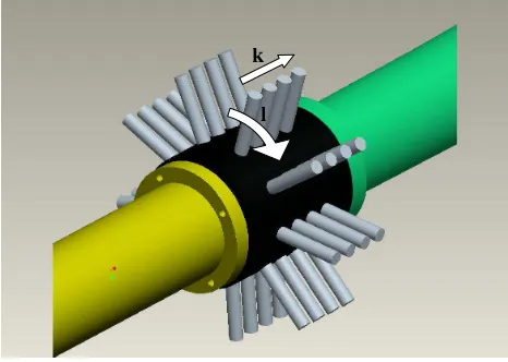
discussed in Holste and Neise.29 _{For a particular pressure measurement, ˆp}

l,k, wherel is the circumferential

coordinate andkthe axial coordinate, as shown in figure 2, a frequency response function can be calculated using any reference pressure (or the signal to the speaker), and used to calculate the modified (normalised by the reference pressure) azimuthal mode, as per equation (11). The benefit of using a frequency response function as opposed to the complex pressure is two-fold: firstly, flow noise, which is significant due to the fan, may be reduced; secondly, if the reference pressure is from another microphone, as opposed to the speaker for example, then a calibration procedure may be used to account for frequency response differences between different microphones.

To expand out equation (11) for the purposes of clarity, equations (13) and (14) show how for a particular axial location,k, the modified azimuthal modes (−4 to +4) may be calculated via a matrix inversion. This procedure needs to be repeated for different axial locations; a minimum of two to determine incident and reflected amplitudes. Furthermore, for the mode (-1), for example, as the second radial mode amplitude is an additional unknown,viz. (-1,0) and (-1,1), a minimum of four axial locations are required, for the incident and reflected amplitudes.

Once the modified azimuthal modes in the circumferential direction have been acquired for each axial location, the second stage is carried out, using equation (12). An expansion of this equation is shown in equation (15) and (16) and consists for a second time of setting up a system of linear equations for which the unknowns may be solved by matrix inversion.

                                                                   ˆ p_0,k ˆ pref

ˆ p1,k ˆ pref

ˆ p2,k ˆ pref

ˆ p_3,k ˆ pref

ˆ p4,k ˆ pref

ˆ p5,k ˆ pref

ˆ p6,k ˆ pref

ˆ p_7,k ˆ pref

ˆ p8,k ˆ pref                                                                    =                            

e[−4j(0∗ 2π

9)] e[−3j(0∗ 2π

9)] e[−2j(0∗ 2π

9)] e[−1j(0∗ 2π

9 )] e[0j(0∗ 2π

9)] e[+1j(0∗ 2π

9)] e[+2j(0∗ 2π

9)] e[+3j(0∗ 2π

9)] e[+4j(0∗2π 9)]

e[−4j(1∗ 2π

9)] e[−3j(1∗ 2π

9)] e[−2j(1∗ 2π

9)] e[−1j(1∗ 2π

9 )] e[0j(1∗ 2π

9)] e[+1j(1∗ 2π

9)] e[+2j(1∗ 2π

9)] e[+3j(1∗ 2π

9)] e[+4j(1∗2π 9)]

e[−4j(2∗ 2π

9)] e[−3j(2∗ 2π

9)] e[−2j(2∗ 2π

9)] e[−1j(2∗ 2π

9 )] e[0j(2∗ 2π

9)] e[+1j(2∗ 2π

9)] e[+2j(2∗ 2π

9)] e[+3j(2∗ 2π

9)] e[+4j(2∗2π 9)]

e[−4j(3∗ 2π

9)] e[−3j(3∗ 2π

9)] e[−2j(3∗ 2π

9)] e[−1j(3∗ 2π

9 )] e[0j(3∗ 2π

9)] e[+1j(3∗ 2π

9)] e[+2j(3∗ 2π

9)] e[+3j(3∗ 2π

9)] e[+4j(3∗2π 9)]

e[−4j(4∗ 2π

9)] e[−3j(4∗ 2π

9)] e[−2j(4∗ 2π

9)] e[−1j(4∗ 2π

9 )] e[0j(4∗ 2π

9)] e[+1j(4∗ 2π

9)] e[+2j(4∗ 2π

9)] e[+3j(4∗ 2π

9)] e[+4j(4∗2π 9)]

e[−4j(5∗ 2π

9)] e[−3j(5∗ 2π

9)] e[−2j(5∗ 2π

9)] e[−1j(5∗ 2π

9 )] e[0j(5∗ 2π

9)] e[+1j(5∗ 2π

9)] e[+2j(5∗ 2π

9)] e[+3j(5∗ 2π

9)] e[+4j(5∗2π 9)]

e[−4j(6∗ 2π

9)] e[−3j(6∗ 2π

9)] e[−2j(6∗ 2π

9)] e[−1j(6∗ 2π

9 )] e[0j(6∗ 2π

9)] e[+1j(6∗ 2π

9)] e[+2j(6∗ 2π

9)] e[+3j(6∗ 2π

9)] e[+4j(6∗2π 9)] e[−4j(7∗

2π

9)] e[−3j(7∗ 2π

9)] e[−2j(7∗ 2π

9)] e[−1j(7∗ 2π

9 )] e[0j(7∗ 2π

9)] e[+1j(7∗ 2π

9)] e[+2j(7∗ 2π

9)] e[+3j(7∗ 2π

9)] e[+4j(7∗2π 9)]

e[−4j(8∗ 2π

9)] e[−3j(8∗ 2π

9)] e[−2j(8∗ 2π

9)] e[−1j(8∗ 2π

9 )] e[0j(8∗ 2π

9)] e[+1j(8∗ 2π

9)] e[+2j(8∗ 2π

9)] e[+3j(8∗ 2π

9)] e[+4j(8∗2π 9)]                                                                       

h−4,k

h−3,k

h−2,k

h−1,k

h_0,k

h1,k

h2,k

h_3,k

h4,k

                                           (13)                                           

h−4,k

h−3,k

h−2,k

h−1,k

h0,k

h1,k

h_2,k

h3,k

h4,k

                                           =                            

e[−4j(0∗ 2π

9)] e[−3j(0∗ 2π

9)] e[−2j(0∗ 2π

9)] e[−1j(0∗ 2π

9 )] e[0j(0∗ 2π

9)] e[+1j(0∗ 2π

9)] e[+2j(0∗ 2π

9)] e[+3j(0∗ 2π

9)] e[+4j(0∗2π 9)]

e[−4j(1∗ 2π

9)] e[−3j(1∗ 2π

9)] e[−2j(1∗ 2π

9)] e[−1j(1∗ 2π

9 )] e[0j(1∗ 2π

9)] e[+1j(1∗ 2π

9)] e[+2j(1∗ 2π

9)] e[+3j(1∗ 2π

9)] e[+4j(1∗2π 9)]

e[−4j(2∗ 2π

9)] e[−3j(2∗ 2π

9)] e[−2j(2∗ 2π

9)] e[−1j(2∗ 2π

9 )] e[0j(2∗ 2π

9)] e[+1j(2∗ 2π

9)] e[+2j(2∗ 2π

9)] e[+3j(2∗ 2π

9)] e[+4j(2∗2π 9)]

e[−4j(3∗ 2π

9)] e[−3j(3∗ 2π

9)] e[−2j(3∗ 2π

9)] e[−1j(3∗ 2π

9 )] e[0j(3∗ 2π

9)] e[+1j(3∗ 2π

9)] e[+2j(3∗ 2π

9)] e[+3j(3∗ 2π

9)] e[+4j(3∗2π 9)] e[−4j(4∗

2π

9)] e[−3j(4∗ 2π

9)] e[−2j(4∗ 2π

9)] e[−1j(4∗ 2π

9 )] e[0j(4∗ 2π

9)] e[+1j(4∗ 2π

9)] e[+2j(4∗ 2π

9)] e[+3j(4∗ 2π

9)] e[+4j(4∗2π 9)]

e[−4j(5∗ 2π

9)] e[−3j(5∗ 2π

9)] e[−2j(5∗ 2π

9)] e[−1j(5∗ 2π

9 )] e[0j(5∗ 2π

9)] e[+1j(5∗ 2π

9)] e[+2j(5∗ 2π

9)] e[+3j(5∗ 2π

9)] e[+4j(5∗2π 9)] e[−4j(6∗

2π

9)] e[−3j(6∗ 2π

9)] e[−2j(6∗ 2π

9)] e[−1j(6∗ 2π

9 )] e[0j(6∗ 2π

9)] e[+1j(6∗ 2π

9)] e[+2j(6∗ 2π

9)] e[+3j(6∗ 2π

9)] e[+4j(6∗2π 9)]

e[−4j(7∗ 2π

9)] e[−3j(7∗ 2π

9)] e[−2j(7∗ 2π

9)] e[−1j(7∗ 2π

9 )] e[0j(7∗ 2π

9)] e[+1j(7∗ 2π

9)] e[+2j(7∗ 2π

9)] e[+3j(7∗ 2π

9)] e[+4j(7∗2π 9)]

e[−4j(8∗ 2π

9)] e[−3j(8∗ 2π

9)] e[−2j(8∗ 2π

9)] e[−1j(8∗ 2π

9 )] e[0j(8∗ 2π

9)] e[+1j(8∗ 2π

9)] e[+2j(8∗ 2π

9)] e[+3j(8∗ 2π

9)] e[+4j(8∗2π 9)]                             −1                                                                    ˆ p0,k ˆ pref

ˆ p_1,k ˆ pref

ˆ p2,k ˆ pref

ˆ p3,k ˆ pref

ˆ p4,k ˆ pref

ˆ p_5,k ˆ pref

ˆ p6,k ˆ pref

ˆ p7,k ˆ pref

ˆ p_8,k ˆ pref                                                                    (14) ˆ pref               

h−1,x0

h−1,x1

h−1,x2

h−1,x3

               =             e(

−jk+_x,−1,0x0)_C−

1,0J−1(kr,−1,0a) e(+jk −

x,−1,0x0)_C−

1,0J−1(kr,−1,0a) e(

−jk+_x,−1,1x0)_C−

1,1J−1(kr,−1,1a) e(+jk −

x,−1,1x0)_C−

1,1J−1(kr,−1,1a)

e(−jk + x,−1,0x1)

C−1,0J−1(kr,−1,0a) e(+jk − x,−1,0x1)

C−1,0J−1(kr,−1,0a) e(−jk + x,−1,1x1)

C−1,1J−1(kr,−1,1a) e(+jk − x,−1,1x1)

C−1,1J−1(kr,−1,1a)

e(−jk +

x,−1,0x2)_C−

1,0J−1(kr,−1,0a) e(+jk −

x,−1,0x2)_C−

1,0J−1(kr,−1,0a) e(−jk +

x,−1,1x2)_C−

1,1J−1(kr,−1,1a) e(+jk −

x,−1,1x2)_C−

1,1J−1(kr,−1,1a)

e(−jk +

x,−1,0x3)_C−

1,0J−1(kr,−1,0a) e(+jk −

x,−1,0x3)_C−

1,0J−1(kr,−1,0a) e(−jk +

x,−1,1x3)_C−

1,1J−1(kr,−1,1a) e(+jk −

x,−1,1x3)_C−

1,1J−1(kr,−1,1a)

                           ˆ a+−1,0

ˆ a−−1,0

ˆ a+−1,1

ˆ a−_−1,1

               (15)                ˆ a+−1,0

ˆ a−_−1,0

ˆ a+−1,1

ˆ a−−1,1

              

= ˆ_pref

           

e(−jk +

x,−1,0x0)_C−

1,0J−1(kr,−1,0a) e(+jk −

x,−1,0x0)_C−

1,0J−1(kr,−1,0a) e(−jk +

x,−1,1x0)_C−

1,1J−1(kr,−1,1a) e(+jk −

x,−1,1x0)_C−

1,1J−1(kr,−1,1a)

e(

−jk+_x,−1,0x1)_C−

1,0J−1(kr,−1,0a) e(+jk −

x,−1,0x1)_C−

1,0J−1(kr,−1,0a) e(

−jk+_x,−1,1x1)_C−

1,1J−1(kr,−1,1a) e(+jk −

x,−1,1x1)_C−

1,1J−1(kr,−1,1a)

e(

−jk+_x,−1,0x2)_C−

1,0J−1(kr,−1,0a) e(+jk −

x,−1,0x2)_C−

1,0J−1(kr,−1,0a) e(

−jk+_x,−1,1x2)_C−

1,1J−1(kr,−1,1a) e(+jk −

x,−1,1x2)_C−

1,1J−1(kr,−1,1a)

e(−jk +

x,−1,0x3)_C−

1,0J−1(kr,−1,0a) e

(+jk−_x,−1,0x3)_C−

1,0J−1(kr,−1,0a) e

(−jk+_x,−1,1x3)_C−

1,1J−1(kr,−1,1a) e

(+jk−_x,−1,1x3)_C−

1,1J−1(kr,−1,1a)

            −1               

h−1,x0

h−1,x1

h−1,x2

h−1,x3

IV.

Spatial Coherence of Acoustic Modes

The coherence function γ2

ij(f) of two quantities i(t) and j(t) is the ratio of the square of the absolute

value of the cross-spectral density function to the product of the auto-spectral density functions of the two quantities:

For all f, the quantity γ2

ij(f) satisfies 0≤γ2ij(f)≤1. As discussed in Bendat and Piersol30 page 172,

for example, the situation where the coherence function is greater than zero but less than unity may be explained by one of the following three possible physical situations.

• Extraneous noise is present in the measurements.

• The system relating i(t) and j(t) is not linear.

• j(t) is an output due to an input i(t) as well as to other inputs.

However, if i(t) andj(t) are simply unrelated, the coherence will be zero. It is this latter point which is exploited in this technique. A modal decomposition performed in one region in the duct can be related to a second modal decomposition at a different axial region. As the modal decomposition separates the sound field into complex values the magnitudes of which are related to the modal magnitudes, cross- and auto-modal spectra can be defined from which a coherence can be determined. It would be expected that the coherence would be high when modal orders are common to both regions and low when neither or only one mode has a significant magnitude.

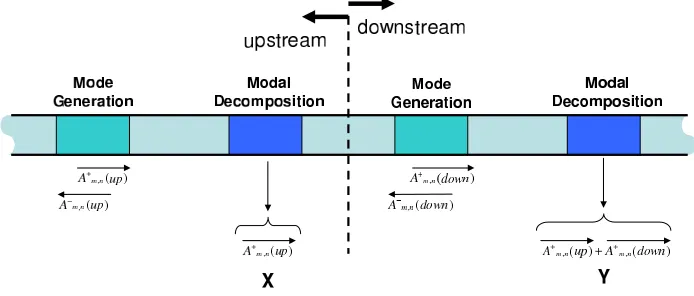
In order to test this hypothesis, a test scenario depicted in figure 3 was examined. In turbomachinery, acoustic modes can be generated through rotor/stator interaction as discussed by Tyler and Sofrin.31 _The

test scenario might represent mode generation by a single rotor/stator pair, followed by additional mode generation by a second single rotor/stator pair downstream in the duct. With reference to figure 3, this will result in modes A+

mn and A

−

mn propagating in the forward and rearward directions respectively. A modal

decomposition of forward travelling modes performed at location X will identify A+

mn(up) only whereas

a second modal decomposition of forward travelling modes, performed at Y, will identify A+

mn(up) and

A+

mn(down) also. Calculating the coherence between locationsX andY on amodal basis, identifies whether

modes have been generated upstream or downstream of locationX, as the coherence;

Figure 3. Schematic for numerical evaluation of coherence based modal decomposition technique.

γ2_X+_,Y+= high forA+_mn(up) ⇒A+_mn(up) generated upstream (17)

γ2_X+_,Y+= low forA+_mn(down) ⇒A+_mn(down) generated downstream or not present (18)

γ_A2±

m,n(X),A

±

m,n(Y)=

|G_A±

m,n(X),A

±

m,n(Y)|

2

G_A±

m,n(X),A

±

m,n(X)GA

±

m,n(Y),A

±

m,n(Y)

(19)

where,

|G_A±

m,n(X),A

±

m,n(Y)|

2_{= [A}±

m,n(X)]

∗

∗A±m,n(Y) (20)

G_A±

m,n(X),A

±

m,n(X)=|A ±

m,n(X)|2 (21)

G_A±

m,n(Y),A

±

m,n(Y)=|A ±

m,n(Y)|

2 ₍₂₂₎

(23)

the techniques could be applied to the simulated data upon calculation of the complex modal coefficients.

A. Simulated Data

1. Sound Field Generated by a Single Point Monopole Source in a Hard Walled Annular Flow Duct

The frequency-domain Green’s function for a duct with an axial irrotational mean flow must satisfy

∇2−Mx2

∂2

∂x2 −2ikMx

∂ ∂x+k

2

G (x,y) =−δ(x−y) (24)

and for a hard-walled boundary condition

∂G

∂n = 0 (25)

wherenis a unit vector normal to the surface of the duct.

Following the formulation of Goldstein32_{the sound pressure generated at position (x, r, ϕ) due to a single}

monopole source with volume velocityq0=v0A located at (xq0, rq0, ϕq0) can be expressed as

p(⇆₎

(x, r, ϕ|xq0, rq0, ϕq0) =−jωρq0g(

⇆₎

(x, r, ϕ|xq0, rq0, ϕq0) (26)

=q0

ρc

2

∞

X

m=−∞

∞

X

n=0

Jm(σmnr/R) Jm(σmnrq0/R) αmnNmn

e−im(φ−φq0) e−ik

±

mn(x−xq0) (27)

whereq0is the source volume velocity,ρandcare the density and speed of sound of the propagation medium.

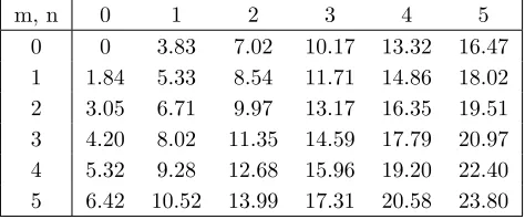
2 Equation (27) provides the pressure distribution in the duct as a function of frequency when the duct is excited by a single monopole source located on the duct surface. For this case, all duct modes are excited. As each mode is associated with a cut-on frequency dependent on the eigenvalue σmn, the frequency can

be expressed in a dimensionless form known as the Helmholtz number. The Helmholtz numbers associated with some of the first radial modes are given in table 1.

m, n 0 1 2 3 4 5

0 0 3.83 7.02 10.17 13.32 16.47 1 1.84 5.33 8.54 11.71 14.86 18.02 2 3.05 6.71 9.97 13.17 16.35 19.51 3 4.20 8.02 11.35 14.59 17.79 20.97 4 5.32 9.28 12.68 15.96 19.20 22.40 5 6.42 10.52 13.99 17.31 20.58 23.80

Table 1. Table of Helmholtz numbers for modeskR

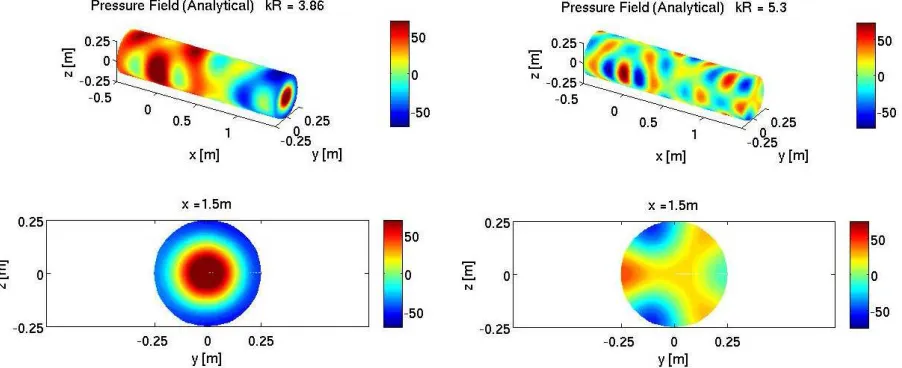
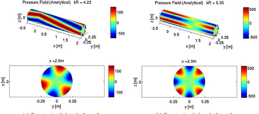
Figure 4(a) shows a solution to equation 27 for a Helmoltz number just above the Amn=A0,1 cut-on.

As the modal magnitudes are greatest just above the cut-on values, we can see this mode is dominant over

8 of 18

the other modes present in the duct. In figure 4(b) we see the pressure distribution in the duct at a higher Helmholtz number, showing the complex nature of the sound field excited by the monopole.

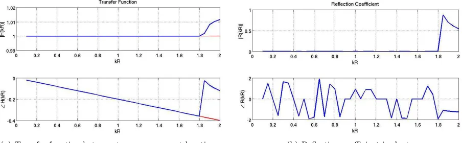
As the modal decomposition technique of section B separates the radial modes into incident and reflected parts, a simple two-measurement transfer function technique such as that developed by Chung and Blaser33 was calculated to verify the uni-directional nature of the simulated data. Figure 5(a) shows the transfer function between two measurement locations of equal azimuthal angle separated by 0.05min a simple duct of radius 0.25mexcited by a monopole source located at (x, φ, r) = (0,0,0.25). The reflection coefficient of figure 5(b) demonstrates that the analytical formulation of equation 27 is indeed uni-directional, although this is only verified for the plane wave region.

A modal decomposition of the pressure field excited by a monopole source is given in figure 6. To be seen in the top plot are the azimuthal modes. Of note is the fact thatAm=A0 Am =A1 both contain radial

contributions, cutting on at Helmholts numbers of 3.83 and 5.33 respectively. The lower two plots show the full radial decomposition in both incident and reflected directions for Helmholtz numbers up to 6.

Although no additional flow velocity is incorporated into the simulations, figure 7 shows, with a Mach number equal to 0.5, how the pressure field is modified upstream and downstream of the monopole location when the axial wave numbers are adjusted to account for added mean flow.

2. Sound Field Generated by Multiple Point Monopole Sources in a Hard Walled Annular Flow Duct

For the purposes of demonstrating the source location technique, specific modes needed to be excited up-stream and downup-stream of the duct in figure 3. This can be achieved by locating multiple sources around the duct and by adjusting their phases appropriately using the expressions of equation 28. The total sound field is found through superposition of equation 27 for each source.

q(θl) =qme(im 2πl

S ) where

l= 0,1, . . . ,(S−1);

θl=

2πl S

(28)

Figures 8, 9, 10, 11, show the pressure field in a simple duct for different target azimuthal modes.

V.

Results

Referring again to figure 3, an initial test set up with A±

m(up) = A

±

+2 and A

±

m(down) = A

±

+3 was

simulated. The results of the upstream modal decomposition are shown in figure 12(a). The configuration for the “microphone” arrays are four axial locations separated by 0.05m of ten sensors equispaced around the circumference of the 0.5m diameter duct. To be seen is how only the A++2 is detected in the incident

field but how the downstreamA−

+3 mode is measured in the reflected field. When a modal decomposition is

performed downstream, figure 12(b) shows both A++2 andA++3 are measured in the incident field and how

there is no significant modal magnitude reflected from downstream of this position.

To calculate the coherence according to equation 19 will result in unity in the absence of averaging. In addition, as the results of the numerical simulation are so exact the modes upstream and downstream are identical for all Helmholtz numbers including those where the modes are not cut-on. In order to repre-sent a more realistic test environment, the complex pressure fields generated with equations 27 and 11 are transformed into the time domain according to the equation

p(t) =

6

X

kR=0

ℜhpˆ(x)∗e(jkRRct)

i

(29)

An example of the process for two sample pressure locations is shown in figure 13 where just a single Helmholtz number is displayed.

Table 2. Spectral estimate parameters

Parameter Value

Segment length, i.e., data points per segment, N p 600

Sample rate, fsamp, Hz 2,610 (2∗kR(max) = 12)

Segment length,Td=N p/fsamp, s 0.2299

Sampling interval, ∆t= 1/fsamp, s 3.8314X10−4

Frequency step, ∆f = 1/Td, Hz 4.35 (∆kR= 0.0199)

Upper frequency limit, fc= 1/(2∆t) =fsamp/2, Hz 1305 (kR= 6)

No. of frequencies, Ly=fc/∆f =N p/2 300

No. of independent samples 20

Overlap 0

Returning to the test set-up of figure 12, a result of the coherence calculated between Amn=A+_2,0(X) andAmn=A+2,0(Y) is shown. Here we see that as the this mode is common to both regions the coherence

is high above the cut-on for that mode.

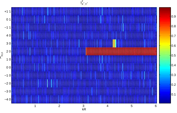
If the coherences are calculated between each mode pair the results can be displayed in the form shown in figure 15. This presentation is extremely informative as common modes can be immediately identified and hence the power of the technique is underlined. Two further test set-ups are examined in figures 16 and 17.

(a) Pressure distribution in a duct just above theAmn=A0,1 cut-on Helmholtz number..

(b) Pressure distribution in a duct at a higher Helmholtz num-ber, showing complex nature of the sound field.

Figure 4. Excitation of all acoustics modes using single monopole source.

VI.

Conclusions

A technique has been presented which can be used to determine the plane at which an acoustic radial mode is generated in a duct when modal decomposition is achievable at multiple locations in the duct. The technique might be used in aero-engines to help locate noise sources and modal scattering. An spatial coherence is defined which may be performed on a modal basis. A proof of concept was carried out using simulated data of known modal structure. The results validate the technique and further development will be carried out where coherence will be measured between single upstream measurements and downstream modes. It is intended that the technique will be tried with full scale engine test data.

10 of 18

(a) Transfer function between two measurement locations. (b) Reflection coefficient in duct.

Figure 5. Characterization of reflection for numerical simulation.

0 20 40 60

|Aplus(kR)|

Azimuthal Modes Decomposition (Incident)

0 20 40 60

|Aplus(kR)|

Radial Modes Decomposition (Incident)

0 1 2 3 4 5 6 0

2 4 6 8x 10

−5

kR

|Aminus(kR)|

Radial Modes Decomposition (Reflected)

(0,0)

( ±1,0)

( ±2,0)

(±3,0)

(±4,0)

(±1,1)

( 0,1) Modes 0

Modes ±1 Modes ±2 Modes±3 Modes ±4

Figure 7. Effect of mean flow on pressure distribution in a duct excited by a single monopole source.

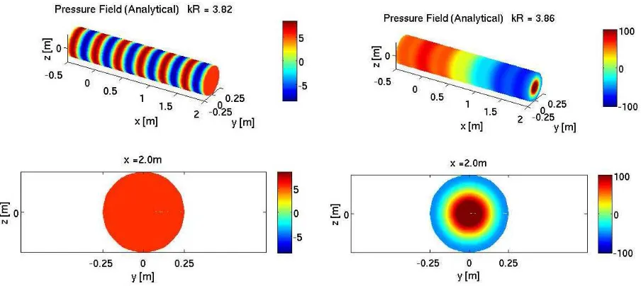
(a) Target azimuthal mode Am = A0. Helmholtz number belowA0,1cut-on.

(b) Target azimuthal mode Am = A0. Helmholtz number aboveA0,1 cut-on.

Figure 8. Numerical simulation using 8 monopole sources distributed equally around the duct surface at same axial location.

12 of 18

(a) Target azimuthal mode Am = A1. Helmholtz number belowA1,1 cut-on.

(b) Target azimuthal mode Am = A1. Helmholtz number aboveA1,1 cut-on.

Figure 9. Numerical simulation using 8 monopole sources distributed equally around the duct surface at same axial location.

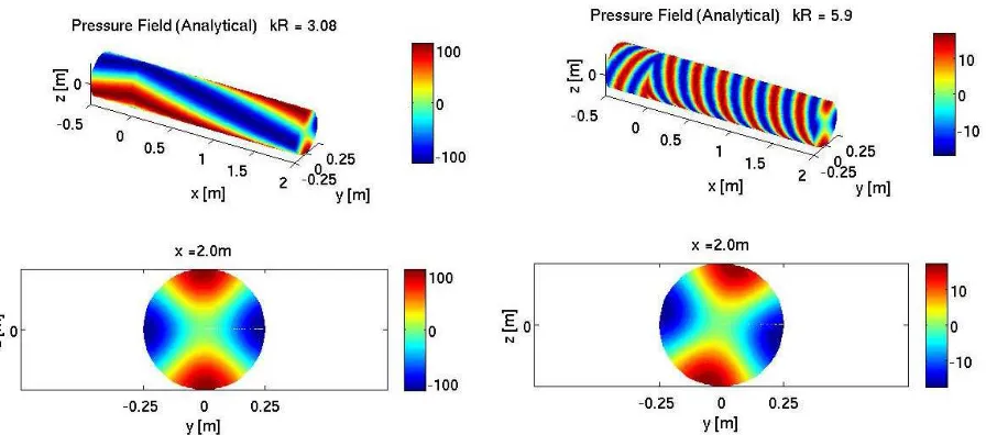
(a) Target azimuthal modeAm=A2. Low Helmholtz num-ber.

(b) Target azimuthal modeAm =A2. A higher Helmholtz number demonstrates the increase in spinning velocity.

(a) Target azimuthal modeAm=A3. (b) Target azimuthal modeAm=A4.

Figure 11. Numerical simulation using 8 monopole sources distributed equally around the duct surface at same axial location.

(a) Modal decomposition of radial modes upstream. (b) Modal decomposition of radial modes downstream.

Figure 12. Modal decomposition results in a duct excited according toA±m(up) =A

±

+2 andA

±

m(down) =A

±

+3.

0 0.5 1 1.5 2 2.5 3 3.5

x 10−3

−1.5 −1 −0.5 0 0.5 1 1.5

Time [s]

Pressure [Pa]

p(t)

x [m]

phi [rads]

ˆ p(x)

−2.50 −2 −1.5 −1 −0.5 0 0.5 1 1.5 2 2.5

1 2 3 4 5 6

−1 −0.5 0 0.5

Figure 13. Example of time domain transform at two complex pressure measurements for a single frequency.

14 of 18

0 1 2 3 4 5 6 0

0.1 0.2 0.3 0.4 0.5 0.6 0.7 0.8 0.9 1

γ2 A+

2,0(X),A + 2,0(Y)

kR

Coherence

Figure 14. Coherence betweenAmn=A +

2,0(X) and Amn=A +

2,0(Y)forA

±

m(up) =A

±

+2 andA±m(down) =A

±

+3 test

set-up.

1 2 3 4 5 6

−4 0 −3 0 −2 0 −1 0 0 0 1 0 2 0 3 0 4 0 −1 1 0 1 +1 1

kR

Am,n

γ2 X+,Y+

0.1 0.2 0.3 0.4 0.5 0.6 0.7 0.8 0.9

Figure 15. Coherence betweenA+

mn(X)andA +

mn(Y)forA

±

m(up) =A

±

+2 andA

±

m(down) =A

±

1 2 3 4 5 6 −4 0

−3 0 −2 0 −1 0 0 0 1 0 2 0 3 0 4 0 −1 1 0 1 +1 1

kR

Am,n

γ2 X+,Y+

0.1 0.2 0.3 0.4 0.5 0.6 0.7 0.8 0.9

Figure 16. Coherence betweenA+mn(X)andA +

mn(Y)forA

±

m(up) =A

±

+3 andA±m(down) =A

±

+4 test set-up.

1 2 3 4 5 6

−4 0 −3 0 −2 0 −1 0 0 0 1 0 2 0 3 0 4 0 −1 1 0 1 +1 1

kR

Am,n

γ2 X+,Y+

0.1 0.2 0.3 0.4 0.5 0.6 0.7 0.8 0.9

Figure 17. Coherence betweenA+mn(X)andA +

mn(Y)forA

±

m(up) =A

± −2 andA

±

m(down) =A

±

+4 test set-up

16 of 18

Acknowledgements

This work was partly supported by the Seventh Framework Programme TEENI project which is funded under EU Commission grant agreement 212367. The help of Mr. Hao Liu in the processing of data for this paper is acknowledged.

References

1_{Karchmer, A. M. and Reshotko, M., “Core noise source diagnostics on a turbofan engine using correlation and coherence}

techniques,” Tech. Rep. TM X-73535, NASA, 1976.

2_{Karchmer, A. M., Reshotko, M., and Montegani, F. J., “Measurement of far field combustion noise from a turbofan engine}

using coherence function,”AIAA 4th Aeroacoustics Conference, No. AIAA-77-1277, Atlanta, Georgia, October 3-5 1977. 3

Reshotko, M. and Karchmer, A. M., “Core noise measurements from a small general aviation turbofan engine,” Tech. Rep. TM81610, NASA, 1980.

4

Halvorsen, W. G. and Bendat, J. S., “Noise Source Identification Using Coherent Output Power Spectra,”Sound and Vibration, Vol. 9, No. 8, 1975, pp. 15, 18–24.

5

Karchmer, A. M., “Conditioned pressure spectra and coherence measurements in the core of a turbofan engine,” Tech. Rep. TM82688, NASA, 1981, AIAA Paper 81-2052.

6_{Shivashankara, B. N., “High bypass ratio engine noise component separation by coherence technique,”AIAA 7th}

Aeroa-coustics Conference, No. AIAA-81-2054, Palo Alto, October 5-6 1981.

7_{Shivashankara, B. N., “High bypass ratio engine noise component separation by coherence technique,”Journal of Aircraft,} Vol. 23, No. 10, 1986, pp. 763–767.

8_{Chung, J. Y., “Rejection of flow noise using a coherence function method,”J. Acoust. Soc. Am., Vol. 62, No. 2, 1977,} pp. 388–395.

9_{Hsu, J. S. and Ahuja, K. K., “A coherence-based technique to separate ejector internal mixing noise from farfield}

measurements,”AIAA/CEAS 4th Aeroacoustics Conference, No. AIAA-98-2296, June 2-4 1998.

10_{Minami, T. and Ahuja, K. K., “Five-microphone method for separating two different correlated noise sources from}

farfield measurements contaminated by extraneous noise,” AIAA/CEAS 9th Aeroacoustics Conference, No. AIAA-03-3261, South Carolina, May 12-14 2003.

11_{Nance, D. K., Separating Contributions Of Small-Scale Turbulence, Large-Scale Turbulence, And Core Noise From}

Far-Field Exhaust Noise Measurement, Ph.D. thesis, Georgia Institute of Technology, 2007.

12_{Bennett, G. J. and Fitzpatrick, J. A., “A comparison of coherence based acoustic source identification techniques,”12th}

International congress on sound and vibration, No. 950, Lisbon, Portugal, 11-14 July 2005.

13_{Bennett, G. J. and Fitzpatrick, J. A., “Noise-source identification for ducted fan systems,”AIAA Journal, Vol. 46, No. 7,} 2008, pp. 1663–1674.

14

Bennett, G. J., Mahon, J., and Fitzpatrick, J., “Non-linear Identification Applied to Broadband Turbomachinery Noise.”

12th CEAS-ASC Workshop, Bilbao, Spain, 2008. 15

Enghardt, L., Zhang, Y., and Neise, W., “Experimental Verification of a Radial mode Analysis Technique Using Wall-Flush Mounted Sensors,”137th Meeting of the Acoustical Society of America, Berlin, March 1999.

16

Enghardt, L., Tapken, U., Neise, W., Kennepohl, F., and Heinig, K., “Turbine Blade/Vane Interaction noise: acoustic mode analysis using in-duct sensor rakes,”7th AIAA/CEAS Conference on Aeroacoustics., No. AIAA-2001-2153, Maastrict, The Netherlands., May 2001.

17

Enghardt, L., Tapken, U., Kornow, O., and Kennepohl, F., “Acoustic Mode Decomposition of Compressor Noise un-der Consiun-deration of Radial Flow Profiles.” 11th AIAA/CEAS Aeroacoustics Conference, No. AIAA-2005-2833, Monterey, California, May 23-25 2005.

18

Tapken, U. and Enghardt, L., “Optimization of Sensor Arrays for Radial Mode Analysis in Flow Ducts,” 12th AIAA/CEAS Aeroacoustics Conference, No. AIAA-2006-2638, Cambridge, MA., May 08-10 2006.

19

Enghardt, L., Holewa, A., and Tapken, U., “Comparison of Different Analysis Techniques to Decompose a Broadband Ducted Sound Field in its Mode Constituents,” 13th AIAA/CEAS Aeroacoustics Conference, No. AIAA-2007-3520, Rome, Italy, May 21-23 2007.

20

Tapken, U., Enghardt, L., and Kennepohl, F., “Radial Mode Analysis of Compressor Noise using different Wall-flush mounted Sensor Arrays.”14th AIAA/CEAS Aeroacoustics Conference, No. AIAA- to be published, Vancouver, Canada, May 5-7 2008.

21

Yardley, P. D., Measurement of Noise and Turbulence Generated by Rotating Machinery, Ph.D. thesis, University of Southampton, 1974.

22_˚

Abom, M., “Modal Decomposition in Ducts Based On Transfer Function Measurements Between Microphone Pairs,” Tech. Rep. Report TRITA-TAK-8702, Department of Technical Acoustics, Royal Institute of Technology, Stockholm, Sweden, 1987.

23

Mungur, P. and Gladwell, G. M. L., “Acoustic wave propagation in a sheared fluid contained in a duct,” Journal of Sound and Vibration, Vol. 9, 1969, pp. 28–48.

24

Munjal, M. L.,Acoustics of Ducts and Mufflers, John Wiley and Sons, 1987.

25_{Kinsler, L. E., Frey, A. R., Coppens, A. B., and Sanders, J. V.,Fundamentals of Acoustics, John Wiley and Sons, 4th} ed., 2000.

27_{Tapken, U., Enghardt, L., Neise, W., and Schimming, P., “Active Control of Noise from Turbomachines-Results of Radial}

Mode Analysis,”Inter-Noise 2001. The 2001 International Congress and Exhibition on Noise Control Engineering, The Hague, The Netherlands, August 2001.

28_{˚Abom, M., “Modal Decomposition in Ducts Based On Transfer Function Measurements Between Microphone Pairs,”}

Journal of Sound and Vibration, Vol. 135, No. 1, 1989, pp. 95–114.

29_{Holste, F. and Neise, W., “Noise Source Identification in a Propfan Model by Means of Acoustical Near Field}

Measure-ments,”Journal of Sound and Vibration, Vol. 203, No. 4, 1997, pp. 641–665.

30_{Bendat, J. S. and Piersol, A. G.,Random Data: Analysis and Measurement Procedures, John Wiley & Sons, 1986.} 31

Tyler, J. M. and Sofrin, T. G., “Axial Flow Compressor Noise Studies,”Society of Automotice Engineers Transactions, Vol. 70, 1961, pp. 309–332.

32_{Goldstein, M. E.,Aeroacoustics, McGraw-Hill Book Company, New York, 1976.}

33_{Chung, J. Y. and Blaser, D. A., “Transfer Function Method of Measuring In-Duct Acoustic Properties. I. Theory.”J.}

Acoust. Soc. Am., Vol. 68, No. 3, 1980, pp. 907–913.

18 of 18