To appear in theInternational Journal of Remote Sensing
Vol. 00, No. 00, Month 20XX, 1–21
Improving specific class mapping from remotely sensed data by cost-sensitive learning
Joel Silvaa∗, Fernando Bacaoa, Maguette Diengd, Giles M. Foodyc, Mario Caetanoab
aNOVA Information Management School, Universidade Nova de Lisboa, Lisboa, Portugal. bDire¸c˜ao Geral do Territ´orio, Lisboa, Portugal.
cSchool of Geography, University of Nottingham, Nottingham, UK.
dFaculty of Sciences and Techniques, University Cheikh Anta Diop, Dakar, Senegal.
(v4.2 released February 2014)
In many remote sensing projects one is usually interested in a small number of land cover classes present in a study area and not in all the land cover classes that make-up the landscape. Previous studies in supervised classification of satellite images have tackled specific class mapping problem by isolating the classes of interest and combin-ing all other classes into one large class, usually called others, and by developcombin-ing a bi-nary classifier to discriminate the class of interest from the others. Here, this approach is called focused approach. The strength of the focused approach is to decompose the original multi-class supervised classification problem into a binary classification prob-lem, focusing the process on the discrimination of the class of interest. Previous studies have shown that this method is able to discriminate more accurately the classes of interest when compared with the standard multi-class supervised approach. However, it may be susceptible to data imbalance problems present in the training data set, since the classes of interest are often a small part of the training set. A result the classification may be biased towards the largest classes and, thus, be sub-optimal for the discrimination of the classes of interest. This study presents a way to minimise the effects of data imbalance problems in specific class mapping using cost-sensitive learning. In this approach errors committed in the minority class are treated as being costlier than errors committed in the majority class. Cost-sensitive approaches are typically implemented by weighting training data points accordingly to their impor-tance to the analysis. By changing the weight of individual data points, it is possible to shift the weight from the larger classes to the smaller ones, balancing the data set. To illustrate the use of the cost-sensitive approach to map specific classes of interest, a series of experiments with weighted support vector machines classifier and Landsat Thematic Mapper data were conducted to discriminate two types of mangrove forest (high-mangrove and low-mangrove) in Saloum estuary, Senegal, a United Nations Ed-ucational, Scientific and Cultural Organisation World Heritage site. Results suggest an increase in overall classification accuracy with the use of cost-sensitive method (97.3%) over the standard multi-class (94.3%) and the focused approach (91.0%). In particular, cost-sensitive method yielded higher sensitivity and specificity values on the discrimination of the classes of interest when compared with the standard multi-class and focused approaches.
Keywords:Support vector machines; land cover mapping; specific class mapping; remote sensing; Landsat; cost-sensitive learning
1. Introduction
Supervised classification has become an important method to derive land cover information from remotely sensed imagery (Mountrakis et al. 2011). One significant advantage of supervised classification is that it allows tailoring the classification process in order to obtain a map depicting only the classes of interest (Foody et al. 2006). Indeed, users are often not interested in a complete characterisation of the landscape but rather on a sub-set of the classes existing in the study area. For example, the analysis may have to be focused on mapping urban classes (Feng et al. 2015; Cockx et al. 2014), abandoned agriculture (Alcantara et al. 2012), specific tree species (Foody et al. 2005; Atkinson et al. 2007), invasive wetland species (Laba et al. 2008), and mangrove ecosystems (Lee and Yeh 2009; Vo et al. 2015). Fundamentally, the accurate discrimination of some classes is more important than the discrimination of others for some applications.
When users are only interested in a sub-set of the classes present in the study area, the use of conventional multi-class supervised classification may be sub-optimal for the purpose (Foody 2004). One of the reasons for this situation has to do with the classification algorithm fine-tuning process. This procedure, necessary in many classification algorithms, consists of finding the parameterisation that yields the maximum overall classification accuracy, that is to find the parameterisation that best discriminates all classes of the classification problem (Hastie et al. 2009). The common approach often seeks, by cross-validation grid-search, to maximise the overall classification accuracy, rather than the specific accuracy in the classification of particular classes. However, the parameterisation that yields the highest overall classification accuracy may not be necessarily the best to discriminate the classes of interest, since these are usually only a small part of the problem (Lark 1995). Indeed, overall accuracy is only one component of classification quality assessment and may not be suited to the requirements of a particular study (Lark 1995). Thus the conventional multi-class supervised classification algorithm is neither tuned nor trained to discriminate the classes of interest, since the class composition of the training set contains all classes regardless of their interest in the analysis and the tuning process searches for the best parameterisation in that larger problem.
The literature shows that there are essentially two alternatives to the standard multi-class supervised approach: one-class learning algorithms and the binarisation strategy (Krawczyk 2015; Galar et al. 2011; Tax 2001).
With the one-class learning algorithms, the user adopts a one-class learning al-gorithm to develop a classifier to identify a single class of interest (e.g. Sanchez-Hernandez et al. 2007; Mack et al. 2014). In this approach only training data belonging to the class of interest is utilised to develop the classifier, which is its most attractive feature in terms of focusing effort and resources on the class of in-terest. However, the one-class classifier may not always be the best approach, since only data about one class is available and thus only one side of the discriminative boundary can be determined (Tax 2001). It can then be difficult to determine how tightly the boundary should fit in all directions around the data in feature space. To overcome this difficulty some one-class classifiers (e.g. support vector data de-scription) assume that the non-interest class has a particular distribution around the class of interest. When the true distribution deviates from the assumption, the method may underperform. That deviation however can only be assessed with training points outside of the class of interest (Tax 2001).
interest from all irrelevant classes (Krawczyk et al. 2015; Fernandez et al. 2013; Galar et al. 2011; Boyd et al. 2006). As binary classification is well-studied, bi-nary decomposition of multi-class classification problems have attracted significant attention in machine learning research and has been shown to perform well in most multi-class problem (Krawczyk et al. 2015). Indeed, binary decomposition has been widely used to develop multi-class SVM showing better generalisation ability than other multi-class SVM approaches (Hsu and Lin 2002). The possibility to parallelise the training and testing of the component binary classifiers is also a big advantage in favour of binarisation apart of their good performance (Galar et al. 2011). In particular, binarisation can be achieved by combining all land cover classes of no interest into a large nominal class, called for example ‘others’ (Foody et al. 2007). In this way the class of interest can be regarded as the positive class and all others as the negative class in the binary classification scenario. Previous studies (Lee and Yeh 2009; Foody et al. 2007; Boyd et al. 2006) have shown it to be possible to decompose the multi-class classification problem in a series of small binary classification problems and achieve results that are more suitable for the particular users’ requests, namely the improvement of the discrimination of partic-ular land cover classes of interest. Although specific class mapping can potentially be a better approach compared to the multi-class supervised classification, it has some particular difficulties, namely data imbalance in the training set. This is be-cause often the classes of interest are only on a small component of the study area (Lark 1995). In fact, applying directly a binary decomposition to the classification problem may result in a highly unproportional allocation of training points to the negative class, leading to imbalance in the training data set (Bishop 2006).
Learning from imbalanced data sets is an important and challenging problem in knowledge discovery in many real-world applications (He and Garcia 2009). Learning from imbalanced data means learning from data in which the classes have unequal numbers of training data points (He and Yunqian 2013). Although there are several degrees of data imbalance, there is no agreement or standard concerning the exact degree of class imbalance required to have a negative effect in the learning process. The central issue with learning from imbalanced data sets is the effect of this condition on the performance of most standard learning algorithms (Kotsiantis et al. 2006). Indeed, most learning algorithms aim to derive the simplest classifier that best fits the training data; this can represent a serious challenge to the development of classifiers with imbalanced data, since such classifier is often biased towards the majority class (Fernandez et al. 2013; Japkowiciz N. 2002). For example, a classifier that omits a large proportion of the minority class cases can yield high overall accuracy, although it may underperform in the discrimination of that class. When trained with this type of data sets, learning algorithms usually fail to accurately learn the distributive characteristics of the data and, consequently, may provide inaccurate results (Lopez et al. 2012). A balanced data set is, therefore, a desirable feature of the training set.
methods are commonly known as cost-sensitive learning (Hastie et al. 2009). In cost-sensitive learning, misclassifications are not treat equally. Data points are assigned a weight representing their relative value: more weight accredits more value. By assigning more weight to a particular data point than to another, the analyst is highlighting its relative importance, and thus informing the learning algorithm that an error in the former is costlier than an error in the latter (Xan-thopoulos and Razzaghi 2014). This additional information directs the learning process to the under-represented classes and thus minimises the effect of learning in imbalanced datasets. In this paper a support vector machine (SVM) classifier is used to demonstrate the use of cost-sensitive learning to minimise the effects of data imbalances in specific class mapping.
Although data imbalance in the training set has been recognised as an important factor in the learning process and is common in natural resource applications using remotely sensed data (Mellor et al. 2015), little attention has been given to its effects and errors in land cover mapping. Thus studies reporting its effects, or esti-mating its effects from previous studies, are rare in literature. Examples addressing data imbalance in remote sensing have been reported mostly in tree species classifi-cation problems. In Baldeck et al. (2015) authors explore the use of standard SVM and biased SVM classification of three tropical tree species using airborne imag-ing spectroscopy. To mitigate the effects of data imbalance, the authors carefully tuned the classification algorithm using the harmonic mean between sensitivity and specificity of the classes of interest, also known as F-score. In Graves et al. (2016) authors examine the effects of data imbalance in the supervised classification of tree species in eight reported studies and address the problem in a twenty-class classification problem. The authors conclude that species with more training data points were consistently over-predicted while species with fewer data points were under-predicted. In Sheeren et al. (2016), authors explore the multiple classifica-tion methods for tree species identificaclassifica-tion in temperate forests using Formosat-2 satellite image time series, reporting that minority classes were often the most con-fused. Thus, data imbalance problems are occurring in application studies where classifications are being used to infer information about land cover.
In this study to demonstrate the effects of data imbalance in the training set and how to mitigate them using cost-sensitive learning, two experiments were con-ducted: first, artificially generated data set was used to illustrate the effects of data imbalance in the development of a classifier.
Second, a series of experiments are presented in a study area located in the Saloum estuary, Senegal. Two land cover classes were defined as the classes of interest. These were classes of mangrove forest that differ in height: high-mangrove and low-mangrove. The distinction between these two classes is important since the transition from high-mangrove to low-mangrove is often a symptom of mangrove degradation (Vo et al. 2015; Dieng et al. 2014).
The innovations presented in this article are three-fold: first, cost-sensitive learn-ing is presented as a way to mitigate problems associated with the use of an im-balanced training set in specific class mapping. In other words, this applicational study intents not only to show that imbalance data sets can undermine the map-ping process, but also to show that cost-sensitive learning can minimise its effects. Second, three classes were used, the two classes of mangrove constituting the classes of interest and the class “others”. This is relevant since the definition of more than one class of interest requires a process to combine the different outcomes of several binary classifiers which is not always trivial and was not fully addressed in previous studies, that have typically focused on a single class. Third, it is shown that the classifier parameterisation is an important step in specific class mapping and more accurate classifiers can be obtained using class specific metrics instead of an overall classification metrics, as is commonly utilised.
2. Classification with imbalanced data sets
Learning with an imbalanced data set is one of the most challenging problems in many real-world applications and it has been recognised as a crucial problem in machine learning and data mining (Cao et al. 2013; Chawla 2005). Class imbal-ance problems may occur when the training set is not evenly distributed among the classes (Chawla 2005). There is no agreement, or standard, concerning the exact degree of class imbalance required for a dataset to lead to a biased classifier (He and Yunqian 2013). This uneven condition is usually quantified by the ratio between the size of the minority class and the size of the majority class, usually called bal-ance ratio (Weiss 2004). Data set balbal-ance ratios can vary greatly, for example from 1:1 (balance data set) to extreme cases such as 1:100 or more (e.g. Weiss 2004). In Weiss and Provost (2003), a 26 binary-class datasets were analysed showing how class imbalance impacts minority class classification performance. The results sug-gest that class imbalance leads to poorer performance when classifying data points belonging to the minority class. Geometrically, a classifier developed with a im-balanced training set pushes the discrimination boundary away from the majority class, bring it closer to the minority class He and Yunqian (2013). This happens because by pushing the boundary away from the majority class toward to minority class, the number of misclassifications on the majority class are minimised, which is the term that contributes the most for the overall classification error. This impact can be quite severe, as datasets with class imbalances between 1:5 and 1:10 can have a minority class error rate more than 10 times that of the error rate on the majority class (Weiss and Provost 2003). This suggests that datasets with even moderate levels of class imbalance (e.g. 1:2) can suffer from class imbalance issues (He and Yunqian 2013).
Most classifiers assume the classes present in the training set contain the same or similar number of data points (Xanthopoulos and Razzaghi 2014). Since classi-fication algorithms are designed to generalise from data and output the simplest classifier that best fits the training data, classifiers will then typically seek to max-imise overall accuracy, and thus tend to underperform on imbalanced data sets (Akbani et al. 2004).
manip-ulating the classes’ distributions in the training data set either by over-sampling the minority class or by under-sampling the majority class (Qiao and Zhang 2013). In other words, in these methods data points are added to the minority class or re-moved from the majority class to balance the training set. There are however some issues with these procedures. Over-sampling may, for example, render longer train-ing time and over-fitted classifiers (Rahman and Davis 2014; He and Garcia 2009). Since over-sampling, at its simplest way, appends replicated data to the original data set, the algorithm may become too specific and may not generalise well (Jap-kowiciz N. 2002). Under-sampling, on the other hand, may remove important data points for class discrimination (Chawla 2005). The methods on the second group, on the other hand, adapt a classification algorithm to bias towards the minority class, for example defining a cost function that penalises more misclassifications committed on data points of the minority class. The training data set is then balanced by shifting the weight of the training set from the larger classes to the smallest. These methods are generally named as cost-sensitive learning methods (Xanthopoulos and Razzaghi 2014). A way to implement the cost-sensitive ap-proach is by incorporating the weight of data points weight in the SVM classifier (Xanthopoulos and Razzaghi 2014).
2.1. Weighted support vector machine
The SVM is a popular supervised classification algorithm that has been successfully applied in many domains (Shalev-Shwartz and Ben-David 2014). In particular, in the classification of remotely sensed imagery, the study and application of SVM is extensive and well known (Mountrakis et al. 2011). In its origin, the SVM was developed to solve binary classification problems with linearly separable classes. However, SVM was extended with the introduction of the kernel trick and slack variables to solve non-linearly separable classes (Deng et al. 2012). The use of ker-nels allowed the SVM to solve non-linear problems by mapping the original data points into a higher dimensional space where a linear classifier is able to discrimi-nate them (Shawe-Taylor and Cristianini 2004). The introduction of slack variables, on the other hand, relaxed the original SVM optimisation problem; a non-zero slack variable allows a particular data point to not meet the margin requirement at a cost proportional to its magnitude, allowing some training data points to be misclassified (Xanthopoulos and Razzaghi 2014). This version is usually known as soft-margin SVM. The corresponding optimisation problem is formulated as follows (Shawe-Taylor and Cristianini 2004):
min w,ξ
1 2w
Tw+CeTξ (1)
subject to yi(wTφ(xi) +b)≥1−ξi fori= 1. . . m whereyi is the label of thei-th
data point xi of the training set, b is the bias term,m is the number of training
2004):
min
α
1 2
X
i,j
αiαjyiyjK(xi,xj)− X
i
αi (2)
subject toP
iyiαi= 0 and 0≤αi ≤C fori, j = 1. . . m, whereαiare the Lagrange
multipliers, K(xi,xj) = φT(xi)φ(xj), quantifies the similarity between two
arbi-trary training data points, xi and xj in the kernel space. The index variables i
and j both ranging from 1 to m to define a pairwise combination of training data points.
Note that under these conditions, the Lagrange multipliers are bounded by the parameter C and thus all misclassifications of training cases are penalised in the same amount. This might not be appropriate especially if the data set is imbal-anced. For example, when trained with imbalanced data sets in which the number of negative instances outnumbers the positive instances, the performance of SVM may drop significantly (Yang et al. 2007). Indeed, SVM may end up classifying all testing data set as belonging to the majority class (Zhang et al. 2015). The optimisation problem (2) tries to minimise first term, responsible to maximise the margin between the support vectors, and the second term, responsible to minimise the number of misclassified training cases. The regularisation parameter C defines the trade-off between maximising the margin and minimising the classification er-ror in the training set (Hwang et al. 2011). Thus, if C is not large enough, SVM learns to classify everything as belonging to the negative class, since that makes the margin larger with maximum accuracy in the training set (Xanthopoulos and Razzaghi 2014).
A way to adapt the SVM approach to cost-sensitive learning is by increasing the trade-off parameter C associated to the minority class (Hwang et al. 2011; Xanthopoulos and Razzaghi 2014). With the weighted support vector machines (WSVM) each data point is assigned a particular weight value; this weight is usually associated to some class characteristic such as size (Hwang et al. 2011). The original SVM problem is then reformulated in the following way:
min w,ξ
1 2w
Tw+CσTξ (3)
subject to yi(wTφ(xi) + b) ≥ 1−ξi for i = 1. . . m, where σ is the vector of
weights. The user can then set different weights to different data points according to a predetermined criterion. Applying the KKT conditions, the original WSVM problem can be reformulated in its dual form:
min
α
1 2
X
i,j
αiαjyiyjK(xi,xj)− X
i
αi (4)
subject to P
iyiαi = 0 and 0 ≤ αi ≤ Cσi for i, j = 1. . . m where αi are the
(a) (b) (c) (d)
(e) (f) (g) (h)
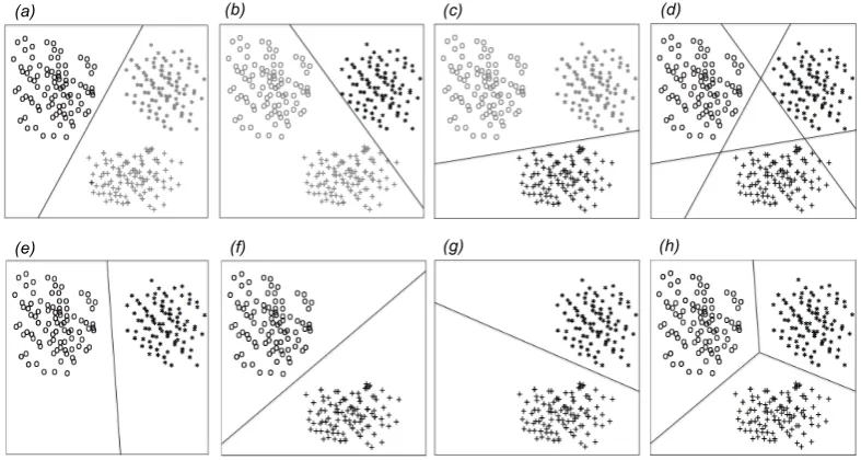
Figure 1. Binary decomposition of multi-class problem. The frames represent the scatter plot in the feature space of three different classes: circles, stars and crosses. OVR strategy in frames (a), (b), (c) and (d) and OVO strategy in frames (e), (f), (g) and (h).
by the inverse of its correspondent class size. In this way, the misclassifications of elements belonging to the majority class receive proportionally less importance than those belonging to the minority class. Note that if data set is balanced, the number of negative data points equals the number of positive data points. Thus the WSVM with this weighting rule reduces to non-weighted SVM.
2.2. Combining binary classifiers
Like SVM, WSVM is at its core a binary classifier. If one wants to apply the WSVM to a multi-class problem, the two more common strategies are (Chang and Lin 2011; Galar et al. 2011): the one-vs-rest (OVR) (figure 1 frames (a), (b), (c) and (d)) and the one-vs-one (OVO) (figure 1 frames (e), (f), (g) and (h)).
The OVR strategy breaks the multi-class classification down into a series of binary classification problems where each class is in turn compared with all others (Shalev-Shwartz and Ben-David 2014). In this way, aN-class classification problem is decomposed into N binary classification problems. For example, in a three-class classification problem, a first classifier is developed to discriminate the class in black (frame (a)) from all other classes are combined into a single class, in grey. The process is then repeated for the other two classes (frames (b) and (c)). The final step is then performed either by assigning the class with positive outcome or by selecting the class with the largest decision value (Rifkin and Klautau 2004) (frame (d)). However, if the label-assigning rule is not based on the decision value directly, some data points may not be classified, because it is possible for a point to be rejected from all classes (Shalev-Shwartz and Ben-David 2014). The OVR strategy is may be susceptible to class imbalances even if the training set is balanced, since the negative class is effectively composed by all other classes combined into one large class (Bishop 2006).
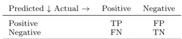
[image:8.595.94.488.52.262.2]Table 1. Binary confusion matrix.
Predicted↓Actual→ Positive Negative
Positive TP FP
Negative FN TN
Classification is then done by inputting the data point into each particular binary classifier and labelling by majority voting. In this way, if there are N classes, the number of binary classifiers is then 12N(N −1) (Shalev-Shwartz and Ben-David 2014) (frame (h)). Although the number of binary classification problems is of the orderN2 and may represent a significant memory requirement this solution, it may also provide simpler models (less support vectors), and thus improve generalisation (Deng et al. 2012). Which strategy is the best is a still an on-going debate (Chang and Lin 2011; Galar et al. 2011).
2.3. Comparison and evaluation of classifiers
The design and implementation of a learning algorithm require the use of accuracy metrics to assess the quality and compare the performance of alternative classi-fiers. For example, when fine-tuning a classification algorithm, it is often necessary to compute an accuracy metric to determine the parameterisation that yields on average the highest accuracy value. Although commonly used, the overall classi-fication accuracy (the proportion of correctly classified data points) may not a reliable metric when the training set is imbalanced. This is because the majority class dominates the behaviour of this metric, and thus it gives optimistically biased results (Xanthopoulos and Razzaghi 2014). Indeed, the definition of the accuracy metric is particular important for binary classification, since the performance of the classifiers can be particularly sensitive to the classes’ relative size (Xanthopoulos and Razzaghi 2014; Shalev-Shwartz and Ben-David 2014). In this conditions, the results of the fine-tuning process may be unreliable not because of the process but rather because of the accuracy metric employed in the process. If the training data set is unbalanced and the classification accuracy is utilised, the outcome of the fine-tuning process will indicate that a particular parameterisation is the one with the highest classification accuracy but may indeed biased towards the majority class, since that parameterisation may yield a classifier that classifies very accurately the majority class in detriment of the minority class (Hwang et al. 2011). There are better alternative accuracy metrics to the classification accuracy specially when the data set is imbalanced, for example sensitivity and specificity (Hastie et al. 2009). At the basis of this analysis is the binary confusion matrix (table 1).
[image:9.595.199.381.62.101.2]producer’s accuracy of the positive class and specificity is the producer’s class of the negative class. In this way, sensitivity indicates how good the classifier is recog-nizing positive cases and specificity indicates how good the classifier is recognising negative cases (Xanthopoulos and Razzaghi 2014).
Often sensitivity and specificity are combined in one metric for better analysis and comparison (Tang et al. 2009). In particular, the geometric mean between sensitivity (s) and specificity (S) (Kubat and Matwin 1997) in Equation 5 is par-ticularly useful:
G=√sS (5)
The geometric mean (G) indicates the balance between classification perfor-mances on the positive and negative class. High misclassification rate in the positive class will lead to a low geometric mean value, even if all negative data points are correctly classified (Hwang et al. 2011). This is a desirable feature specially when the testing sample is asymmetric. Indeed, it can be prove that, in a binary classifi-cation scenario, classificlassifi-cation accuracy is the weighted average between sensitivity and specificity, where the weights are the proportion of each class in the sample. For example, if 10% of the sample is in the positive class and 90% is located in the negative class, a classifier that simply classifies every data point as belonging to the negative class yields an overall accuracy of 0.90. However, its sensitivity is 0.0 and specificity 1.0, and thus geometric mean G is 0.0. In this way, if both sensitivity and specificity are high, the geometric mean G is also a high value; but if one of the component accuracies, sensitivity or specificity, is low, the geometric mean G is affected by it. Note that in some cases a testing sample has to be asymmetric, that is, one class has more testing data points than the other, simply due to its variability. This is the case in a class specific mapping problem, where the majority of the study area is typically outside the class of interest and thus contains all other classes. Thus, the geometric mean can be an important accuracy metric for class specific mapping, since it is particularly sensitive to the over-fitting to the negative class (i.e. others class) and to the degree in which the positive class (i.e. class of interest) is neglected (Nguyen et al. 2010).
3. Data and methods
Figure 2. Saloum river delta in Senegal.
high-mangrove and low-mangrove. High-mangrove is generally characterised by a dense and tall canopy, while low-mangrove tends to show less dense and decayed canopy. In this study area, high-mangrove class is composed by species like Rhi-zophora racemose, Rhizophora mangle and Avicennia Africana (Diop 1986), and low-mangrove by Sesuvium portulacastrum,Sporobolus robustus,Paspalum vagina-tum, and Philoxerus vermicularis (Diop 1986).
The Saloum river delta was designated a United Nations Educational, Scientific and Cultural Organization (UNESCO) World Heritage site for its remarkable nat-ural environment and extensive biodiversity and is listed in the Ramsar List of Wetlands of International Importance (Mitsch and Gosselink 2015). Particularly important is Saloum’s mangrove system, occupying roughly 180 000 ha supporting a wide variety of fauna and flora, and the local economy (Mitsch and Gosselink 2015).
Remotely sensed data of the study area were acquired on 26 November 2010 by Landsat 5 Thematic Mapper (TM) and downloaded from United States Geological Survey (USGS) Global Visualisation web site. In this study all non-thermal bands (bands 1 to 5 and 7) have been used. Since only one image was utilised for analysis and the atmosphere may be considered to be homogeneous within the study area, atmospheric correction was not necessary (Song et al. 2001) and, thus, the classi-fication was performed using the original image digital numbers. In the same year of the image acquisition, fieldwork and aerial imagery interpretation were under-taken to derive ground-reference data. This analysis showed that the study area is composed by six large land cover classes: water, high-mangrove, low-mangrove, bare soil, savannah and shrubs. The training set comprised of 180 pixels per class (= 30 times the number of discriminatory variables) for each of the six land cover classes.
Table 2. Summary of the different experiments: experiments with (*) indicate benchmark. SSVM represents the standard use of SVM; FSVM represents the focused approach with SVM; FOVO represents the focused approach with cost-sensitive and OVO; and FOVR the focus approach with cost-sensitive and OVR.
Experience Training set Fine-tuning Imbalanced Cost-sensitive Strategy
SSVM(*) All classes General No No OVO
FSVM(*) Three classes Specific Yes No OVR
FOVO Three classes Specific Yes Yes OVO
FOVR Three classes Specific Yes Yes OVR
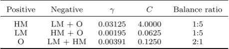
Table 3. Parameterisation using focused approach. Positive Negative γ C Balance ratio
HM LM + O 0.03125 4.0000 1:5 LM HM + O 0.00195 0.0625 1:5 O LM + HM 0.00391 0.1250 2:1
class discrimination. The training set was balanced over all six classes and thus cost-sensitive methodology was not applied. The radial-basis function was chosen as kernel and it was used in all the tested approaches. The free-parametersC and γ of the radial-basis function were determined using a 5-fold cross-validation grid-search with overall accuracy as performance metric. In this way the fine-tuning process is effectively searching for the parameterisation with the highest overall accuracy regardless of the classes. From this analysis the parameters were set as γ = 0.00097 and C = 64. The experiment was conducted using LIBSVM-3.12 (Chang and Lin 2011) software interfaced with MATLABR. This software package
implements the standard SVM, unweighted analysis, with the OVO strategy for multi-class problems (Chang and Lin 2011).
The second benchmark constitutes the focused approach to map specific classes without taking into account the data imbalances present in the training set. This benchmark classification used the standard SVM (e.g. Boyd et al. 2006). For this reason this approach is named where as focus SVM (FSVM). All non-mangrove classes were combined into a large class called ’others’ for use in the training stage. The training set in the analysis is thus composed of three classes: high-mangrove (HM), low-mangrove (LM) and others (O) class. In this way three binary classifiers were developed, each one focusing in the discrimination of one particular class. The geometric mean between sensitivity and specificity was applied in 5-fold cross-validation trials for fine-tuning. Table 3 summarises the parameterisations derived from the fine-tuning analysis and shows the balance ratios to quantify the size difference present in each pair of classes. The balance ratio is the ratio between the sizes of each of the pair. For example, the balance ratio between high-mangrove (180 data points) class and rest of the training set (900 data points) is 1:5. To combine the different outcomes of each classifier, and to avoid non-labelled data points, the assigned label was that of the class with maximum decision value (Shalev-Shwartz and Ben-David 2014). These experiments were conducted with the same software package as in previous experiment.
In contrast with the previous experiment, the fine-tuning does not take the overall classification accuracy as metric but rather the geometric mean between sensitivity and specificity, which is specific of each target class. In this paper, and for clarity, any fine-tuning process that takes into account the overall classification accuracy and not the classification of specific classes will be qualified as general, and specific otherwise.
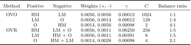
[image:12.595.126.456.92.151.2] [image:12.595.176.406.182.232.2]limi-Table 4. Parameterisation and weights for each pair of classes: using OVO strategy and using OVR strategy.
Method Positive Negative Weights (+, -) γ C Balance ratio OVO HM LM 0.0056, 0.0056 0.00012 1024 1:1
LM O 0.0056, 0.0014 0.00012 128 1:4
O HM 0.0014, 0.0056 0.00098 2 4:1
OVR HM LM + O 0.0056, 0.0011 0.06250 256 1:5 LM HM + O 0.0056, 0.0011 0.00391 8 1:5 O HM + LM 0.0014, 0.0028 0.00098 4 2:1
tations. The first benchmark, although widely used, is not optimised for the dis-crimination of the classes of interest, since the learning algorithm is evaluated on a different class composition than that with was tuned and trained. The second benchmark is an improvement over the first, suggested in previous studies. But, this leads to an classifier developed with an imbalanced data set, which may bias the analysis to the larger classes. Thus the first benchmark, while developed with a balanced training data set, was neither tuned nor trained to discriminate the classes of interest; and the second benchmark, while trained and tuned to discrim-inate the classes of interest, suffers the effects of training data imbalances. The remain approaches tackle these two problems. In other words, they tackle the class specific mapping while avoiding possible data imbalances issues using cost-sensitive learning.
To that end, data point weights were defined as the inverse of its training set size, similar to what has been applied in other studies, such as Xanthopoulos and Razzaghi (2014). In this way by assigning more weight to the data points in the smaller classes, the training set weight distribution shifts from the largest class to the smallest classes minimising the bias towards larger classes. Two approaches were then analysed, one using OVO strategy and another using OVR (table 4).
In FOVO, on the other hand, all classes of no interest were combined into a large one, and thus the training set consisted in only three classes, high-mangrove, low-mangrove and others class. Fine-tuning was specific to each binary classifier and the training data set was imbalanced, and cost-sensitive analysis was employed. The multi-class strategy was the OVO; no reclassification was necessary.
High-mangrove and low-mangrove classes have the same amount of data points (table 4 – Balance ratio), thus the weights associated to their data points is equal, 0.0056. The others class is the majority class, and the weight associated to its data points is thus comparatively smaller to those of high-mangrove and low-mangrove, 0.0014. The free-parameters were fine-tuned using 5-fold cross-validation trials and the experiments were conducted with LIBSVM-weights-3.12 (Chang and Lin 2011) interfaced with MATLABR.
Classification accuracy was estimated using an independent testing set of 100 random pixels per land cover class comprising a total of 600 pixels. An image analyst visually classified each pixel in the same year as the image acquisition with support of Google Earth and fieldwork data. The accuracy of each classification was expressed in terms of the proportion of correctly classified testing data points. Since a single testing set was used for each test site, the statistical significance of the difference in overall accuracy between different classification approaches will be assessed using the McNemar test (Foody 2009).
[image:13.595.127.456.70.148.2]McNe-(a) (b) (c) (d)
Figure 3. Illustration of the effects of data imbalance in the training data set with different degrees of balance ratios. The data set was generated artificially and represents a purposely simple classification problem, projected in the feature space. The minority class represented with crosses and the majority class represented with circles. Straight line is the discrimination plane generated with the non-weighted approach. Dashed line is the discrimination plane generated with the weighted approach. In frame (a) balance ratio is 1:2, in frame (b) is 1:3, in frame (c) is 1:5 and in frame (d) is 1:10.
mar test however focus on proportion of pixels where one classifier was correct but the other was incorrect. The analysis will be based upon the evaluation of the 100(1−α)% confidence interval, where α is the level of significance, for the difference between two accuracy values expressed as proportions (say p1 and p2) expressed as (Fleiss et al. 2003):
p2−p1±zαs (6)
where the term zα is the tabulated Normal distribution value with a level of
sig-nificance of α and s is the standard error derived of the difference between the proportions, which can be determined by (Fleiss et al. 2003):
s=
r
p01+p10−(p01−p10)2
n (7)
here p10 the proportion of testing pixels where the first classifier was correct and the second was incorrect and p01 the proportion of testing pixels where the first classifier was incorrect and the second was correct and n is the number of testing samples. In this way, the statistical assessment of the differences was conducted to determine if these were significantly different or not (Foody 2009).
4. Results and discussion
A sequence of experiments with synthetic data were performed to illustrate the effects of data imbalance in the resulted classifiers. For this purpose two normal distributed classes, the circles and crosses, were artificially generated with the same variability but different class sizes. The classes are linearly separable and thus a linear SVM classification algorithm is capable of developing a classifier without errors in the training data set. That is, it is able to find the optimal discrimination plane. The example is purposely simple to illustrate the effects of data imbalances in the training set. In other words, in real-world applications the relative size between classes is not the only factor contributing to the classification algorithm. The class mean location, variance and overlapping for example are also important informing the learning algorithm.
[image:14.595.100.484.58.132.2]Table 5. Summary of the accuracy results in percentage obtained with each experiment. OA stands for overall accuracy, Ss. for sensitivity and Sp. for specificity, Gm the geometric mean between sensitivity and specificity for each class of interest.
High-mangrove Low-mangrove
Method OA (%) Ss (%) Sp (%) Gm (%) Ss (%) Sp (%) Gm (%)
SSVM 94.3 88.0 95.6 91.7 85.0 96.2 90.4
FSVM 91.0 86.0 92.9 88.9 72.0 94.8 82.6
FOVO 97.3 95.0 97.8 96.4 93.9 98.2 95.6
FOVR 96.7 93.0 97.4 95.2 91.0 97.8 94.3
with different balance ratios. The minority class represented with crosses and the majority class represented with circles. In frame (a) balance ratio is 1:2, in frame (b) is 1:3, in frame (c) is 1:5 and in frame (d) is 1:10. Straight line is the discrim-ination plane generated with the non-weighted approach and dashed line is the discrimination plane generated with the weighted approach. When data sets are not balanced, the discrimination boundary (straight line) is pushed away from the majority class. This gives more room to the majority class to accommodate atypical pixels, that is pixels with low frequency of occurrence or that were not represented in the training data set. However, the decision boundary is closer to the minority class, providing less room to accommodate pixels that deviate from the training data set distribution. Thus, the classifier is overfitted around the minority class. In other words, a point belonging to the minority class that deviates from the training data set distribution may be misclassified, because the discrimination boundary is too close to its true class. Thus, a classifier developed with an imbalanced data set may induce a classification with high number of false negatives in the minority class. That is, the minority class may be underestimated. This explains the findings of previous studies, like Graves et al. (2016), that have shown a trend where classes with more samples were consistently over-predicted while classes with fewer sam-ples were under-predicted. With the discrimination plane induced by the weighted approach, the effects of data imbalanced are mitigated. The training data points were weighted according to its class, using the same rule as presented in section 2.1. Here the decision boundary is further from the minority class compared to the plane induced by the non-weighted approach (straight line). This provides enough room to include atypical pixels, thus mitigating the effects of the overabundance of data points belonging to the majority class. In this way, by controlling the weight of the minority class data points, it is possible to inform the learning algorithm to push away the decision boundary to avoid over-fitting around the minority class.
The overall accuracy yielded by the two benchmarks was 94.3% and 91.0% for SSVM and FSVM, respectively (table 5). The difference in overall accuracy between these two approaches can be attributed mainly to the data imbalance present in the training set used in the FSVM experiment. Indeed, the training set used for SSVM is balanced since the six classes have precisely the same number of data points, in contrast with the FSVM where roughly 66.7% of the training consists in one class (others class), with the rest being equally distributed by high-mangrove and low-mangrove. Then when the binarisation process in FSVM is applied, the binary classifiers used to discriminate the target classes are developed with an imbalanced training set. The imbalance ratio in the training data set for the classes of interest is 1:9.
[image:15.595.106.477.82.149.2]omits more positive cases than SSVM, which are precisely the pixels belonging to the classes of interest. On the other hand, with lower specificity FSVM commits more negative cases (elements of the class of non-interest) to the class of interest. These errors led to a decrease of the geometric mean of 2.8% and 7.8% in the discrimination of high-mangrove and low-mangrove respectively.
It is also important to notice that, although FSVM was tuned using the geometric mean, specific for each class of interest, that was not sufficient to overcome the effects of imbalance data. The determination of the parameters is an important factor in the sense that provides more sensibility to the learning algorithm about the boundaries of the classes of interest. However the issue introduced by the data imbalance remains, since the decision boundary will still be pushed way from the majority class.
The FOVO and FOVR experiments were conducted with the same training set as that of FSVM, but the data imbalance was mitigated with the use of data point weights. Overall accuracies were 97.3% and 96.7% for FOVO and FOVR, respectively, 6.3% and 5.7% higher than the FSVM. Sensitivity and specificity were higher in both classes of interest. The geometric mean yielded by FOVO and FOVR were 7.5% and 6.3% higher, respectively, for high-mangrove and 13.0% and 11.7% higher for low-mangrove. These results show how the use of weighted observations can be used to mitigate the effects of data imbalance in the training set for specific class mapping. In fact, the cost-sensitive approaches (FOVO and FOVR) yielded the highest geometric mean values in the discrimination of the classes of interest.
The main difference between SSVM and the cost-sensitive approaches is on the fine-tuning process, since both data sets are balanced, the first by design and the second by application of data point weights. The fine-tuning process in SSVM is generic; in other words, a single set of parameters was determined as the best set of parameters for the discrimination of each possible pair of classes since the utilised software implements OVO strategy to deal with multi-class problems. Thus, the fine-tuning process is effectively estimating the parameterisation yielding the maximum overall discrimination accuracy for the discrimination of the six land cover classes and not the best parameterisation for the particular discrimination of the classes of interest.
On the other hand, in FOVO and FOVR, the fine-tuning process is specific, that is it was applied to each particular pair of classes, and thus instead of determining the parameters that best fit the discrimination of all classes, each pair of classes had its own particular parameterisation. In contrast with SSVM, the training set and the fine-tuning process applied in FSVM is the same as those utilised in the two cost-sensitive approaches. In FSVM, although the fine-tuning process was specific to each particular binary classification problem, and not global as in SSVM, the imbalances present in the training set were not addressed.
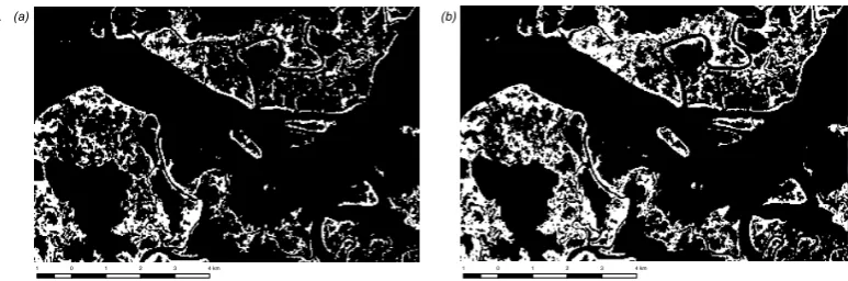
(b) (a)
Figure 4. Binary map showing the areas of high-mangrove (white) and no-high-mangrove (black) classified by the standard SVM (SSVM) frame (a) and the focused SVM with one-vs-one (FOVO) frame (b). Top left corner at (313659,1541131) and bottom right corner (333858,1540057) EPSG 32628.
Table 6. 95% confidence interval (CI) on the estimated dif-ference in overall accuracy (DA) obtained between the ap-proaches. Results are presented in percentage and decision is done at 5% level of significance
Method DA 95% CI for DA Decision SSVM vs. FSVM 3.3 1.7 - 4.9 Different FOVO vs. SSVM 3.0 1.5 - 4.5 Different FOVR vs. SSVM 2.4 1.2 - 3.6 Different FOVO vs. FOVR 0.6 0.3 - 0.9 Equivalent
composition of the training data set and in the way the learning algorithm param-eters were fixed. Concretely, since the class of interest is only one small class in a larger group of six, a set of parameters inducing a classifier that correctly predicts the majority of the classes but neglecting the small class of interest, scores high in fine-tuning process. Such model ultimately defines a decision boundary closer to the class of interest, which may lead to a model that under-predicts this class. In other words, the classifier that is less sensitive to the class of interest. Note that the pixels added by FOVO are located near the interface between the class of interest and its negative. This suggests that these are pixels localised on edge of the class distribution, and thus are more likely to be misclassified by a classifier with low sensitivity to the class of interest, such SSVM. In other words, the classification errors committed by SSVM tend to be localised in such regions. This led the FOVO approach to predict roughly 7.0% more pixels of the classes of interest than the SSVM.
[image:17.595.99.486.47.175.2] [image:17.595.181.403.284.343.2]5. Summary and conclusions
Often users’ interest is on a small sub-set of land cover classes present in the study area and not in a complete characterisation of the landscape. In these cases, conventional supervised classification techniques may not be appropriate for the derivation of information about these classes. Previous studies have shown that by combining the classes of no interest into a large single class and by decomposing the multi-class problem into a series of binary classification problems is sometimes a better approach than the conventional supervised classification method. However, this approach may suffer from data imbalance issues, since the classes of interest are usually a small component of the training set. In this article, cost-sensitive learning was applied to overcome data imbalances problems present in the training data. Experiments were conducted with Landsat 5 Thematic Mapper in Saloum, Senegal, where the classes of interest were high-mangrove and low-mangrove. The cost-sensitive learning outperformed the conventional multi-class approach and the focused approach in the discrimination of each class of interest. Classification ac-curacies derived from cost-sensitive approaches were significantly different from those derived from the standard multi-class and the focused approaches. Cost-sensitive approach also improved class specific discrimination. Indeed, for high-mangrove, the cost-sensitive learning approach yielded sensitivity and specificity geometric mean of 96.4% against 91.7% yielded by the multi-class approach and 88.9% yielded by the focused approach. And for low-mangrove, the cost-sensitive learning approach yielded a geometric mean of 95.6% against 90.4% yielded by the multi-class approach and 82.6% yielded by the focused approach. The cost-sensitive approaches as predicted roughly 7.0% more pixels of the classes of interest than the conventional supervised classification. Since interest was on more that one class, it is necessary to combine the outcomes of several binary classifiers. The two most common approaches, the one-vs-one (OVO) and the one-vs-rest (OVR), were com-pared. The differences between the accuracies derived from OVO and OVR were not statistically significant. Indeed, although OVO show higher classification ac-curacy than OVR (97.3% against 96.7%), OVR acac-curacy was non-inferior to that of OVO at 5% significance level and using a 1.0% zone of indifference. From an operational point of view, the effort to apply OVO or OVR was the same, because the number of classes of interest was small. Since that is the case in most practical cases, the use of OVO or OVR may then be of little if any relevance. In summary, the study results suggest that the cost-sensitive learning is an effective solution to overcome data imbalances present in the training set and thus contribute to improve the classification accuracy of specific mapping of classes of interest.
Acknowledgements
Research by Joel Silva was founded by the ”Funda¸c˜ao para a Ciˆencia e Tecnologia” (SFRH/BD/84444/2012). The authors are grateful to the referees for their helpful comments on the article.
References
Alcantara, C., Kuemmerle, T., Prishchepov, A. V., Radeloff, V. C., 2012. Mapping aban-doned agriculture with multi-temporal MODIS satellite data. Remote Sensing of Envi-ronment 124, 334–347.
Atkinson, P. M., Foody, G. M., Gething, P. W., Mathur, A., Kelly, C. K., 2007. Investigating spatial structure in specific tree species in ancient semi-natural woodland using remote sensing and marked point pattern analysis. Ecography 30 (1), 88–104.
Baldeck, C. A., Asner, G. P., Martin, R. E., Anderson, C. B., Knapp, D. E., Kellner, J. R., Wright, S. J., 2015. Operational tree species mapping in a diverse tropical forest with airborne imaging spectroscopy. PLoS ONE 10 (7).
Bishop, C. M., 2006. Pattern recognition and machine learning, information science and statistics. Springer, Berlin.
Boyd, D., Sanchez-Hernandez, C., Foody, G., 2006. Mapping a specific class for priority habitats monitoring from satellite sensor data. International Journal of Remote Sensing 27 (March 2015), 37–41.
Cao, P., Zhao, D., Zaiane, O., 2013. An Optimized Cost-Sensitive SVM for Imbalanced Data Learning. In: Advances in knowledge discovery and data mining. pp. 280–292. Chang, C.-C., Lin, C.-L., 2011. Libsvm: A library of support vector machines. ACM
Trans-actions on Intelligent Systems and Technology 2, 1–27.
Chawla, N. V., 2005. Data Mining for Imbalanced Datasets: An Overview. Data Mining and Knowledge Discovery Handbook, 853–867.
Cockx, K., Van de Voorde, T., Canters, F., 2014. Quantifying uncertainty in remote sensing-based urban land-use mapping. International Journal of Applied Earth Obser-vation and Geoinformation 31 (1), 154–166.
Deng, N., Tian, Y., Zhang, C., 2012. Support Vector Machines: Optimization Based Theory, Algorithms, and Extensions. CRC Press.
Dieng, M., Silva, J., Goncalves, M., Faye, S., Caetano, M., 2014. The land/ocean interac-tions in the coastal zone of west and central africa, estuaries of the world. estuaries of the world.
Diop, E. S., 1986. Estuaires holoc`enes tropicaux. etude g´eographique physique compar´ee des rivi`eres du sud du saloum (s´en´egal) `a la mellcor´ee (r´epublique de guin´ee). Ph.D. thesis.
Du, S., Chen, S., 2005. Weighted support vector machine for classification. Systems, Man and Cybernetics, 2005 IEEE 2, 859–864.
Faye, S., Diaw, M., Malou, R., Faye, A., 2008. Impacts of climate change on groundwater recharge and salinization of groundwater resources in senegal. Groundwater and climate in Africa proceeding of the Kampala conference.
Feng, X., Foody, G., Aplin, P., Gosling, S. N., 2015. Enhancing the spatial resolution of satellite-derived land surface temperature mapping for urban areas. Sustainable Cities and Society 19, 341–348.
Fernandez, A., Lopez, V., Galar, M., Del Jesus, M. J., Herrera, F., 2013. Analysing the classification of imbalanced data-sets with multiple classes: Binarization techniques and ad-hoc approaches. Knowledge-Based Systems 42, 97–110.
Fleiss, J. L., Levin, B., Paik, M. C., 2003. Statistical methods for rates and proportions; 3rd ed. Wiley Series in Probability and Statistics. Wiley, Hoboken, NJ.
Foody, G. M., 2004. Supervised image classification by MLP and RBF neural networks with and without an exhaustively defined set of classes. International Journal of Remote Sensing 25 (15), 3091–3104.
Foody, G. M., 2009. Classification accuracy comparison: Hypothesis tests and the use of confidence intervals in evaluations of difference, equivalence and non-inferiority. Remote Sensing of Environment 113 (8), 1658–1663.
Foody, G. M., Atkinson, P. M., Gething, P. W., Ravenhill, N. A., Kelly, C. K., 2005. Identification of specific tree species in ancient semi-natural woodland from digital aerial sensor imagery. Ecological Applications 15 (4), 1233–1244.
requirements for the classification of a specific class. Remote Sensing of Environment 104 (1), 1–14.
Galar, M., Fernandez, A., Barrenechea, E., Bustince, H., Herrera, F., 2011. An overview of ensemble methods for binary classifiers in multi-class problems: Experimental study on one-vs-one and one-vs-all schemes. Pattern Recognition 44 (8), 1761–1776.
Graves, S. J., Asner, G. P., Martin, R. E., Anderson, C. B., Colgan, M. S., Kalantari, L., Bohlman, S. A., 2016. Tree species abundance predictions in a tropical agricultural landscape with a supervised classification model and imbalanced data. Remote Sensing In Review, 1–21.
Hastie, T., Tibshinari, R., Friedman, J., 2009. The elements of statistical learning, second edition Edition. Springer Series in Statistics, Springer.
He, H., Garcia, E. A., 2009. Learning from imbalanced data. IEEE Transactions on Knowl-edge and Data Engineering 21 (9), 1263–1284.
He, H., Yunqian, M., 2013. Imbalanced Learning: Foundation, Algorithms and Applica-tions, the instit Edition. John Wiley & Sons, Ltd.
Hsu, C.-W., Lin, C.-J., 2002. A comparison of methods for multiclass support vector ma-chines. IEEE Transactions on Neural Networks 13 (2), 415–425.
Huang Yin-Min, D. S.-X., 2005. Weighted support vector machine for classification with uneven training class sizes. 2005 IEEE International Conference on Systems, Man and Cybernetics 4 (August), 3866–3871.
Hwang, J. P., Park, S., Kim, E., 2011. A new weighted approach to imbalanced data classification problem via support vector machine with quadratic cost function. Expert Systems with Applications 38 (7), 8580–8585.
Japkowiciz N., S. S., 2002. The class imbalance problem: a systematic study. Intelligent Data Analysis 6 (5), 1–39.
Kotsiantis, S., Kanellopoulos, D., Pintelas, P., 2006. Handling imbalanced datasets : A review.
Krawczyk, B., 2015. One-class classifier ensemble pruning and weighting with firefly algo-rithm. Neurocomputing 150 (PB), 490–500.
Krawczyk, B., Wo´zniak, M., Herrera, F., 2015. On the usefulness of one-class classifier ensembles for decomposition of multi-class problems. Pattern Recognition 48 (12), 3969– 3982.
Kubat, M., Matwin, S., 1997. Addressing the Curse of Imbalanced Training Sets: One Sided Selection. In: In Proceedings of the Fourteenth International Conference on Machine Learning. Vol. 4. pp. 179–186.
Laba, M., Downs, R., Smith, S., Welsh, S., Neider, C., White, S., Richmond, M., Philpot, W., Baveye, P., 2008. Mapping invasive wetland plants in the Hudson River National Estuarine Research Reserve using quickbird satellite imagery. Remote Sensing of Envi-ronment 112 (1), 286–300.
Lark, R. M., 1995. Components of accuracy of maps with special reference to discriminant analysis on remote sensor data. International Journal of Remote Sensing 16 (8), 1461– 1480.
Lee, T. M., Yeh, H. C., 2009. Applying remote sensing techniques to monitor shifting wet-land vegetation: A case study of Danshui River estuary mangrove communities, Taiwan. Ecological Engineering 35 (4), 487–496.
Liu, S., Jia, C., Ma, H., 2005. A new weighted support vector machine with GA-based parameter selection. Machine Learning and Cybernetics, 2005. . . . (August), 18–21. Lopez, V., Fernandez, A., Moreno-Torres, J. G., Herrera, F., 2012. Analysis of preprocessing
vs. cost-sensitive learning for imbalanced classification. Open problems on intrinsic data characteristics. Expert Systems with Applications 39 (7), 6585–6608.
Mack, B., Roscher, R., Waske, B., 2014. Can i trust my one-class classification? Remote Sensing 6 (9), 8779–8802.
Mitsch, W., Gosselink, J., 2015. Wetlands. Wiley.
Mountrakis, G., Im, J., Ogole, C., 2011. Support vector machines in remote sensing: A review. ISPRS Journal of Photogrammetry and Remote Sensing 66 (3), 247–259. Nguyen, G. H., Phung, S. L., Bouzerdoum, A., 2010. Efficient SVM training with reduced
weighted samples. Proceedings of the International Joint Conference on Neural Net-works, 1764–1768.
Qiao, X., Zhang, L., 2013. Distance-weighted Support Vector Machine.
Rahman, M. M., Davis, D. N., 2014. Transactions on Engineering Technologies: Special Volume of the World Congress on Engineering 2013. Springer Netherlands, Dordrecht, Ch. Semi Supervised Under-Sampling: A Solution to the Class Imbalance Problem for Classification and Feature Selection, pp. 611–625.
Rifkin, R., Klautau, A., 2004. In defense of one-vs-all classification. Journal of Machine Learning Research 5, 101–141.
Sanchez-Hernandez, C., Boyd, D. S., Foody, G. M., 2007. One-class classification for map-ping a specific land-cover class: SVDD classification of fenland. IEEE Transactions on Geoscience and Remote Sensing 45 (4), 1061–1072.
Sch¨olkopf, B., Smola, A. J., Williamson, R. C., Bartlett, P. L., 2000. New support vector algorithms. Neural computation 12 (5), 1207–1245.
Shalev-Shwartz, S., Ben-David, S., 2014. Understanding Machine Learning: From Theory to Algorithms. Cambridge University Press, New York, NY, USA.
Shawe-Taylor, J., Cristianini, N., 2004. Kernel Methods for Pattern Analysis. Cambridge University Press, New York, NY, USA.
Sheeren, D., Fauvel, M., Josipovi, V., Lopes, M., Planque, C., 2016. Tree Species Classifi-cation in Temperate Forests Using Formosat-2 Satellite Image Time Series, 1–29. Song, C., Woodcock, C. E., Seto, K. C., Lenney, M. P., Macomber, S. A., 2001.
Classi-fication and Change Detection Using Landsat TM Data : When and How to Correct Atmospheric Effects ? Remote Sensing of Environment 75 (00), 230–244.
Tang, Y., Zhang, Y. Q., Chawla, N. V., 2009. SVMs modeling for highly imbalanced clas-sification. IEEE Transactions on Systems, Man, and Cybernetics, Part B: Cybernetics 39 (1), 281–288.
Tax, D. M. J., 2001. One-class classification. Ph.D. thesis.
Vo, T., Kuenzer, C., Oppelt, N., 2015. How remote sensing supports mangrove ecosys-tem service valuation: A case study in Ca Mau province, Vietnam. Ecosysecosys-tem Services 14 (MAY), 67–75.
Weiss, G. M., 2004. Mining with Rarity: A Unifying Framework. SIGKDD Explorations 6 (1), 7–19.
Weiss, G. M., Provost, F., 2003. Learning when training data are costly: The effect of class distribution on tree induction. Journal of Artificial Intelligence Research 19, 315–354. Xanthopoulos, P., Razzaghi, T., 2014. A weighted support vector machine method for
control chart pattern recognition. Computers & Industrial Engineering 70 (October), 134–149.
Yang, X., Song, Q., Wang, Y., 2007. A weighted support vector machine for data clas-sification. International Journal of pattern recognition and artificial inteligence 2 (5), 859–864.