Peptide refinement using a stochastic search

(1)

Peptide Refinement Using A Stochastic Search

Nicole H. Lewis

∗

East Tennessee State University

Johnson City, Tennessee

David B. Hitchcock

University of South Carolina

Columbia, South Carolina

Ian L. Dryden

University of Nottingham

Nottingham, United Kingdom

John R. Rose

University of South Carolina

Columbia, South Carolina

Abstract

Identifying a peptide based on a scan from a mass spectrometer is an important yet highly challenging problem. To identify peptides, we present a Bayesian approach which uses prior information about the average relative abundances of bond cleavages and the prior probability of any particular amino acid sequence. The proposed scoring function is composed of two overall distance measures, which measure how close an observed spectrum is to a theoretical scan for a peptide. Our use of our scoring function, which approximates a likelihood, has connections to the generalization presented by Bissiri et al. (2016) of the Bayesian framework. A Markov chain Monte Carlo algorithm is employed to simulate candidate choices from the posterior distribution of the peptide sequence. The true peptide is estimated as the peptide with the largest posterior density.

KEYWORDS: Stochastic Search, Bayesian Methods, Markov Chain Monte Carlo, Peptide Identification, Tandem Mass Spectrometry

1 Introduction

Proteomics involves the analysis of proteins, particularly their structure, function, abundances, variations, and modifi-cations. In proteomics, scientists begin with the protein and work backwards to determine the gene that is responsible for its production. Proteins are constantly changing and vary with health or disease while a genome remains relatively static. Issues arise in protein identification when an organism’s genome has not been sequenced, more specifically in microbial samples. Only 1%-10% of microbes found in the ecosystem can be cultured. There are countless other microbes that have not been identified and, of the microbes that have been cultured, some will show evidence of post-translational modifications. These post-translational modifications cannot be calculated from the genome (Rose et al., 2010). The area of environmental proteomics has not been fully developed and being able to correctly identify these microbes via protein identification is of great importance especially in ecological samples such as soil and water samples (Schulze, 2004). In clinical proteomics, scientists commonly search for proteins or groups of proteins to help diagnose types of cancers, diseases, or viruses with the goal of early diagnosis. These proteins or groups of proteins can be biomarkers for a disease; see Wulfkuhle et al. (2003), Diamandis (2004), and Visintin et al. (2008). Correctly identifying proteins will also aid in the advance of clinical proteomics.

Current methods for identification of proteins have limitations. With a limited number of known genome sequences, noisy data, and incomplete ion sequences, the accuracy of protein identification requires improvement. In this paper, we describe a Bayesian approach, which aims to improve the identification of proteins.

We employ a Bayesian stochastic search approach to protein identification. We use the prior knowledge of abundances of bond cleavages and the probability of any particular amino acid sequence. Our scoring function combines two

∗_{Nicole H. Lewis, Department of Mathematics and Statistics, East Tennessee State University, Johnson City, TN 37614 (email:}

(2)

measures of distance that measure the closeness of each observed mass-to-charge ratio (m/z) value from a sample to anm/zvalue in a theoretical scan of a peptide. A Markov chain Monte Carlo (MCMC) scheme is utilized to simulate candidate peptides from the posterior distribution, and the peptide with the largest posterior probability is estimated as the true protein. Our approach also allows one to rank the top candidate peptides by their estimated posterior probabilities.

The data come from the Pacific Northwest National Laboratory (PNNL) and can be publicly accessed online for download (Ansong et al., 2011) and is produced by a LTQ Orbitrap yielding doubly charged tryptic peptides. For each peptide, there is a set ofm/zvalues with corresponding intensity values.

1.1 Mass Spectrometry

There are several methods for obtaining the proteomic profile of a sample. With technological advances, mass spec-trometry methods are now more commonly used. Tandem mass specspec-trometry(M S/M S)is a two-stage mass trometry process that allows examination of individual ion fragmentation from a group of ions. Tandem mass spec-trometry is used with an assortment of instruments and scan modes.

Peaks can be identified by plotting the intensities versus a horizontal index, which in proteomic analysis is them/z

value. These peaks characterize the peptide in the sample. The final data spectrum is the line plot of pairs of intensities andm/zvalues (Coombes et al., 2007). Figure 1 pictorially shows the spectrum for a given peptide by plotting the intensity values versus theirm/zvalues. [[Figure 1 goes here]]

1.2 Protein Identification Methods

Presently, there are few methods for identifying protein sequences. A popular approach searches through a database of peptides and then matches the closest peptide using the observed spectrum. Some common algorithms for database searches are MASCOT and SEQUEST (Xu and Ma, 2006). Another approach is de novo sequencing, in which the peptide sequence is determined by recreating a spectrum using the observed spectrum. PepNovo and Peaks are frequently used de novo algorithms (Frank and Pevzner, 2005; Frank, 2009; Ma et al., 2003). A more recent approach, de novo sequencing via probabilistic network modeling, uses a mixture of the other two. In this approach, the de novo method recaptures short peptide sequences and then the peptide sequences are used to refine the search in the database approach (Frank and Pevzner, 2005).

A major concern of the database search and hybrid method is that they rely on the use of a database of peptides. These methods cannot correctly identify the protein if it is not in the database. Some limitations of both the database search and de novo peptide sequencing are lack of accuracy and certainty of the chosen peptides, chemical noise, overly complex fragments, and incomplete ion sequences (Lubec and Afjehi-Sadat, 2007). We introduce a Bayesian model that will aim to improve on the PepNovo approach by identifying the correct peptide without depending on the database of peptides, but instead using more generic prior information.

2 Basic Concepts of Fragmentation

(3)

maintained on the C-terminus, where the C-terminus refers to the end of a peptide that is terminated by a free carboxyl group(−COOH)(IUBMB, 1992, p. 48).

To find the theoretical spectrum, one must first split the true peptide sequence into all possible ion combinations. In practice, we use only thebandyions, although there are several other less common ions. After thebandyions are found, the mass of each ion is determined. The mass for any given ion is found byPK_i=1m(pi) +δ`whereKis the number of amino acids in the ion sequence,pi is the amino acid in theith position,m(pi)is the mass of the amino acid in theith position,`denotes the type of ion such that`∈ {b, y}, andδ`is the offset value for that particular ion type. In tandem mass spectrometry, the peptide fragmentation is determined by offsets that correspond to ion types. That is, the offsets match up to the peaks in a given spectrum, and thus denote the different ion types created in the given mass spectrometer (Danˇc´ık et al., 1999). Since different types of mass spectrometers yield different spectra, Danˇc´ık et al. (1999) developed an offset frequency function that does not depend on instrument type and allows one to define the ion types produced by a given mass spectrometer. The offset value for abion is 0.85 Daltons (Da) and 18.85 Da for ayion.

As an example, consider the peptideQV M ELLQ. There are sixbions and sixyions. The firstbion,Q, has a mass of128.059 + 0.85 = 128.909Da, and the firstyion,Q, has a mass of128.059 + 18.85 = 146.909Da. Continuing with the splitting of the peptide, one obtains the following additionalbions: QV,QV M,QV M E,QV M EL, and

QV M ELLwith masses 227.977, 359.017, 488.060, 601.144, and 714.228 Da, respectively. Similarly, we obtain the following additionalyions:LQ,LLQ,ELLQ,M ELLQ, andV M ELLQwith masses 259.993, 373.077, 502.120, 633.160, and 732.228 Da, respectively. Therefore, the theoretical spectrum for the peptideQV M ELLQis the set of masses: 128.909, 227.977, 359.017, 488.060, 601.144, 714.2284, 732.228, 633.160, 502.120, 373.077, 259.993, and 146.909 Da. Figure 2 shows the theoretical spectrum for the peptideQV M ELLQusing only thebandyions and the positions found above are shown on the(m/z)axis. [[Figure 2 goes here]]

It is important to find the total mass of the peptide because a mass spectrometer will also measure the total mass of the peptide being analyzed. We can use this weight restriction to eliminate peptides that do not have a total mass within a tolerance of the measured mass. The total mass of the peptide is found byPK_i=1m(pi) +mass ofH2O, where the mass of the water molecule is 18.010565 Da. For data that are doubly charged, the total mass becomes PK

i=1m(pi) +mass ofH2O+Hbecause of the second proton that is acquired. The mass of one hydrogen molecule is 1.00794 Da. Thus the total mass for the peptideQV M ELLQis 860.456 Da assuming the data are doubly charged.

3 A Bayesian Model

We propose a Bayesian model with the goal of identifying the true peptide based on the observed spectrum. To identify this true peptide, an MCMC algorithm is used to simulate candidate peptide sequences from an approximate posterior distribution. The motivation will be discussed in Section 3.2.

3.1 Pre-Processing

(4)

3.2 Scoring Function

For our approximate Bayesian model, we first specify a scoring function, which gives a measure of how well the observed spectrum and theoretical spectrum agree. If a candidate peptide’s theoretical spectrum does not align well with the observed spectrum, an overall goodness of fit measure will penalize the candidate peptide. Even after thresh-olding, we still expect there to be noise peaks in the data set and therefore, we incorporate another overall goodness of fit measure that will penalize a candidate peptide when the observed spectrum shows many noise peaks which do not correspond to them/zvalues of the candidates theoretical spectrum. We do know that the mass spectrometer does not always capture every signal peak. Hence, we include an indicator function in our scoring function that signifies the presence or absence of a peak. Our scoring function is an approximation to a generative likelihood with details found in Section 5.1. Our method involves treating the scoring function as if it was a likelihood, even though it is actually an approximate likelihood.

We propose a scoring function of the form

L(X|θ,η, κ1, κ2)∝κ2p1 exp(−κ1S1)κ2t−sexp(−κ2S2) (1)

where our parameter is vectorθ = (τ1b, . . . , τpb, λb1, . . . , λbp, τ y 1, . . . , τ

y p, λ

y 1, . . . , λ

y

p),X contains the observed set of

m/zvalues for a particular spectrum, andηrepresents the string of amino acids for the candidate peptide.S1andS2 are functions ofθandX that are defined below. The other parameters are defined as

• sis the combined number ofbandyions for the candidate peptide

• pis the number ofbions (or equivalently the number ofyions)

• tis the number of peaks in a given candidate peptide

• τb i andτ

y

i are them/zvalues for thebandyion of the candidate peptide

• λb i andλ

y

i ∈ {0,1}are indicator functions that signify whether theithboryion has a corresponding observed peak, wherei= 1, . . . , p

• κ1andκ2represent weights, which play the role of concentration parameters that control how tightly concen-trated the observed peaks are around their corresponding true peaks (see Section 5.1 for more details).

Here,λb_i = 1denotes the presence andλb_i = 0denotes the absence of abion at positioni. Similarly,λy_i = 1denotes the presence andλy_i = 0denotes the absence of ayion at positioni.

Letxj, j= 1, . . . , nT be the observed peaks that are above the thresholdT wherenT represents the number of peaks that are above the thresholdT. We will partition these observed peaks into two sets of signal and noise peaks. In particular letSdenote the set of observed peaks above the thresholdT which are each closest to one of the peaksτk i of the candidate peptide spectrum,i= 1, . . . , pandk∈ {b, y}. We callSthe set of observed signal peaks. LetN be the remaining observed peaks above the thresholdT that are not inS, and we callN the set of observed noise peaks. The goodness of fit measures of the candidate spectrum relative to the observed spectrum are

S1 = p X

i=1

λb_imin

j∈Sd(xj, τ

b i) +λ

y i min

j∈Sd(xj, τ

y i)

(2)

S2 = X

j∈N min

i,k |xj−τ k

i| (3)

andd(xj, τik) = min{|xj−τik|, δ}. We believe that (even allowing for a cushion beyond the usual 0.5 Da threshold, discussed further in Sections 4 and 6, for classifying an observed peak as a true peak) no observed peak will lie beyond 3 Da from the corresponding observed peak. Hence, we chooseδ= 3. This choice works well in practice; note that choosingδmuch larger than this would inflateS1and worsen the performance.

(5)

of the nearest candidate peak to each observed peak. NoteS1is low when the candidate peaks are close to observed peaks, andS2is low when the noise peaks are close to the candidate peaks or if there are fewer noise peaks. When all peaks for the candidate peptide are very close to observed peaks that are above the threshold, thenexp (−S1)is high. When all the observed peaks are close to candidate peaks,exp (−S2)will be high, so thatexp (−S1)andexp (−S2) represent sensitivity and specificity.

Our method has some interesting connections to other Bayes-like approaches. Although our procedure is different from approximate Bayesian computation (ABC), the fact that we are attempting to get close to the similarity scores in the true unobtainable likelihood has similarities with ABC, although there is no simulation in our procedure but rather just a single evaluation of the approximate similarity scores.

An appealing recent work by Bissiri et al. (2016) presents an innovative idea for generalizing the Bayesian paradigm of updating prior beliefs based on observed data. That article gives a framework in which the role of the data is characterized by a loss function involving the data and the parameters (akin to the loss function considered in decision theory). This loss function could be a negative log-likelihood as in the traditional Bayesian setup, but it also could take other forms, so that the practitioner need not specify a formal likelihood as a model for the data. Using this general loss function along with the prior, the prior beliefs are updated to posterior beliefs after the data are observed.

Our method can be connected to this general updating framework nicely, since our scoring function often will not correspond to a generative data model (except in the special case of Laplace noise, when our scoring function in Equation 1 approximates the generative model given later in Equation 10). The negative logarithm of our scoring function in Equation 1 can, however, be viewed as a loss function that measures the closeness of the observed data to a proposed parameter structure. Based on this closeness, the prior belief about the parameter structure (which characterizes the true nature of the peptide) is updated over the steps of the MCMC process, with our eventual goal being the selection of the “best” parameter structure given the posterior belief, which corresponds to the goal in the Bissiri et al. (2016) framework.

3.3 Priors

Huang et al. (2004) estimated the average bond cleavage abundance for each amino acid pair for both thebandyions for gas-phase dissociation spectra. Collision-induced dissociation (CID) fragments the peptides even further during the gas phase in the mass spectrometry process. A cleavage occurs when the peptide bond fragments during collision induced dissociation, and a cleavage pair is theb andy ion pair that are present in the peptide. For example, take the peptideQV M ELLQ. Recall from Section 2 thatQV is one of the sixbions of the peptideQV M ELLQand the complement to thatbion is theyionM ELLQ. These complementary ions are a result of the cleavage between the amino acidsV andM. This information from Huang et al. (2004) will give us insight about when we expect to see cleavages in the pairs of amino acid residues, and thus we use this information to develop prior information about cleavage pair abundance for our Bayesian approach to identify the true peptide.

3.3.1 Cleavage Prior

The cleavage pair abundance prior, denotedπ(λ|β,γ)≡π(λ)is defined as:

π(λ) =

p Y

i=1

P(λb_i, λy_i) (4)

with

P(λb_i =λy_i = 1) =ρby_i ×γi×βi

P(λb_i = 1, λy_i = 0) =ρby_i ×(1−γi)×βi

P(λb_i = 0, λy_i = 1) =ρby_i ×γi×(1−βi)

P(λbi =λ y

i = 0) = 1−ρ by i + [ρ

by

(6)

whereλ= (λb,λy) = (λb1, . . . , λbp, λ y 1, . . . , λ

y p),ρ

by

i is the geometric mean of the average relative abundance of bond cleavages ofbandyions for a particular amino acid pair fori= 1, . . . , pderived from Huang et al. (2004),γiis the probability of the presence of ayion, andβiis the probability of the presence of abion. Here,prepresents the number of cleavage pairs. As a matter of notation, note that our parameter vectorθ(=θγ,β)depends on the values ofγandβ, but our notation will suppress this dependency sinceγandβwill remain fixed throughout the algorithm. Note that the

λb

i’s are modeled as having random marginal Bernoulli distributions with probabilitiesρ by

i βiand theλ y

is are modeled as having random marginal Bernoulli distributions with probabilitiesρby_i γi, andλb

i,λ y

i are all mutually independent for

i= 1, . . . , p. The proof of theλb i’s andλ

y

i’s having a marginal Bernoulli distribution can found in the supplementary material. Figure 3 shows the geometric mean of the average bond cleavage abundance for all cleavage pairs of the

bandyions using Figure 1 in Huang et al. (2004). Note that probabilities for a particular amino acid cleavage pair that are too close to zero may force the algorithm to exclude reasonable peptides. In order for our prior to be more inclusive, we use a linear transformation of the scale used in Huang et al. (2004), of the formρ= 0.49x+ 0.67. Our rescaled distribution has probabilities that range from 0.67 to 1.00. [[Figure 3 goes here]]

3.3.2 Sequence Prior

We now want to specify a prior distribution for a particular sequence (or string) of amino acids in a peptide. The prob-ability of any particular amino acid sequence is represented by the string prior,π(η), which quantifies the probability of a sequence of amino acids appearing consecutively in a peptide sequence. For each amino acid pair in the candidate peptide under consideration, we count how often the pair occurs in the set of known peptides from the same species. Then we find the empirical probability of each amino acid pair using our large database of peptides. Note that one could use other databases that do not contain the current peptide to calculate the empirical probability. The string prior is defined as proportional to the geometric mean ofπ(η_F)andπ(η_R),

π(η)∝pπ(η_F)×π(η_R), (5)

whereπ(η_F)is the joint probability of any particular amino acid sequence calculated from left to right whileπ(η_R)

is the joint probability of any particular amino acid sequence calculated in the reverse direction. Note that this is the geometric mean ofπ(η_F)andπ(η_R). Hereηis the ordered sequence of the amino acids in the current peptide under consideration where the length ofηis the number of amino acids in the candidate peptide, andπ(η)is a probability for this particular sequence. Denote a generic peptide sequence byA1A2· · ·Am−1, wherem−1is the number of amino

acids in the peptide sequence,A0denotes the beginning of the sequence, andAmdenotes the end of the sequence. For example, consider the peptideT GM SN V SK. For this candidate peptide having 8 amino acids,m= 9.π(ηF) is calculated by

π(η_F) =P(A1=a1)× m−1

Y

i=1

P(Ai+1=ai+1|Ai =ai) (6)

with P(A1 = a1) = p1, P[(Ai, Ai+1) = (ai, ai+1)] = pi,i+1, and therefore P(Ai+1 = ai+1|Ai = ai) =

pi,i+1 P

jP[(Ai, Ai+1= (ai, j)]

forj ∈ {A, C, . . . , Y, }whereai represents the amino acid in theith position in the

peptide sequence andam= signifies the termination of a sequence. In a similar manner,π(ηR)is computed by

π(η_R) =P(Am−1=am−1)× m−2

Y

i=0

P(Ai=ai|Ai+1=ai+1) (7)

withP(Am−1=am−1) =pm−1,P(Ai=ai|Ai+1=ai+1) =

pi,i+1 P

jP[(Ai, Ai+1= (j, ai+1)]

forj∈ {A, C, . . . , Y, }

(7)

3.3.3 Prior forκ1,κ2

The concentration parameters,κ1andκ2, are assumed to have independent Gamma(a1,b1) and Gamma(a2,b2) prior distributions respectively, which are independent of the other parameters.

3.4 Posterior

Treating the scoring function as an approximate likelihood, using Bayes’ Theorem, the approximate posterior density can be written as

π(η,λ, κ1, κ2|X)∝L(X|λ,τ,η, κ1, κ2)×π(λ)×π(η,τ)×π(κ1, κ2) (8)

=L(X|θ,η, κ1, κ2)×π(λ)×π(η)×π(κ1, κ2), (9)

whereλ,η, andκ1,κ2are assumed independent. The set ofm/zlocations given byτ = (τ1b, . . . , τpb, τ y

1, . . . , τpy)T is determined by the sequenceη, and soP(τ|η) = 1. Note that this posterior density is only known up to a constant and the actual form of the posterior density is complicated. Therefore, to obtain the posterior probabilities we use MCMC simulation. Our Bayesian method incorporates prior information about the chance of seeing particular cleavage pairs, and also quantifies the prior probability of any particular specific amino acid sequence. We use this posterior density to estimate the true peptide, with candidate peptides having high posteriors being judged more likely to be the true peptide. Our point estimate of the true peptide is the posterior mode, that is, the candidate peptide (among those visited by the search algorithm) with the highest posterior probability, and the posterior distribution variance provides information about the uncertainty of the estimate. Now and henceforth, when we refer to the “posterior,” note that this is an approximation to the true posterior, since our scoring function is an approximation to a true generative likelihood (see Section 5.1 for details).

4 A Markov Chain Monte Carlo Algorithm

Our posterior is complicated and so we employ Markov chain Monte Carlo (MCMC) methods to sample the parameters (Tierney, 1994; Robert and Casella, 1999; Andrieu et al., 2003; Sorensen and Gianola, 2002).

4.1 Initialization

To find a starting peptide for the MCMC algorithm, we only consider candidates with the overall correct mass (within a tolerance). One option is to use an initial iterative sub-algorithm to obtain a starting peptide. Note the actual mass of the true peptide is available to us from the mass spectrometry data, and so we can dramatically reduce the parameter space by searching for peptides with a mass within a specific tolerance (0.5 Da) of the actual mass. To obtain a random starting point, amino acids are randomly added or removed until a peptide is found that has a mass within a tolerance of the mass of the true peptide.

While using the method above will reduce the space of initial peptides, it may still yield a starting peptide far from the truth if the peptide sequence is long, which could result in our method taking a long time to search for the true peptide. Another option for finding a starting peptide is to use the results from PepNovo (Frank and Pevzner, 2005). PepNovo yields a list of the top 2000 best estimated peptides for the true peptide. We can use a peptide from this list as our starting peptide; still ensuring it will have the correct total mass within a tolerance.

4.2 Posterior Simulation

(8)

beginning of the algorithm and are constant throughout the algorithm. Before the algorithm begins, a vectorλcurris generated using theβandγvectors.

MARKOV CHAIN MONTE CARLO ALGORITHM

1. A new peptide is created by randomly replacing one, two, or three amino acids of the current peptide with one, two, or three amino acids. This implies the next candidate peptide will be of the same length or length 1 or 2 shorter or 1 or 2 longer than the current peptide, but will still have a total mass within the tolerance of0.5Da of the true mass.

2. Generate a vectorλnewusing theβandγvectors.

3. Generateκ1 and κ2 from their full conditional distribution: gamma distributions with the shape parameter

α1 =a1+sand scale parameterβ1 =S1+b1and shape parameterα2 =a2+ (t−s)and scale parameter

β2=S2+b2, respectively. Note that the values ofS1andS2are based on the current peptide.

4. Compute the unnormalized posterior probability for both the new and current peptide, computed based on the new and currentλvectors, respectively. Denote these asζ1andζ2, respectively.

5. GenerateU ∼U(0,1). IfU <

_ζ 1

ζ2

×q(λcurr|λnew)

q(λnew|λcurr)

×q(ηcurr|ηnew)

q(η_new|η_curr)

, then the new peptide becomes the

current peptide, andλnewbecomesλcurr. Otherwise, both the current peptide andλcurrremain unchanged. 6. Go to 1.

When exploring large state spaces stochastically, it is important that the algorithm be irreducible: that is, it may visit every potential state with positive probability (Tierney, 1994). To ensure irreducibility, every1000steps we generate an entirely new peptide that is independent of the current state. Note that any sequence with the correct mass has positive probability of being generated in this step (Tierney, 1994).

Steps 1 - 6 are repeated for a large number of iterations. The peptide with the largest posterior density is selected as the estimate of the true peptide, and we retain all generated peptides along with their approximate posterior probabilities (up to a constant).

Trace plots of the log posterior and parameters are used to monitor convergence of the algorithm to determine whether the chain has converged to its stationary distribution and whether the chain is mixing well. Examples of these plots are are shown in Lewis (2013) in Figures 7.4 - 7.6.

To calculate the first proposal densities we need to calculateq(λcurr|λnew)andq(λnew|λcurr). Note thatq(λcurr|λnew) =

q(λcurr)andq(λnew|λcurr) =q(λnew)since the newλis generated independently of the currentλfrom the prior distribution, as described in Section 3.3.1.

To calculate the second set of proposal densities we need to calculateq(η_curr|η_new)andq(η_new|η_curr). Recall from step 1 of the MCMC algorithm, we always replace either one, two, or three amino acids of the current peptide with either one, two, or three amino acids. Hence there is a1/3chance of choosing either one, two, or three amino acids to be replaced. If only one amino acid is chosen to be replaced, then there is a1/nchance that any particular amino acid will be chosen (nrepresents the total number of amino acids in the peptide sequence). If a pair of amino acids is chosen to be replaced, then there is a1/(n−1)chance that a consecutive pair of amino acids will be chosen. If three consecutive amino acids are chosen to be replaced, then there is a1/(n−2)chance that any particular triplet of consecutive amino acids will be chosen.

Also, note that the current and new peptide must have a total mass that is within a tolerance of the total mass of the true peptide. After the number of amino acids to be replaced is fixed, a list of single, pairs, and/or triplets of amino acids is generated such that each has a mass within a tolerance of the mass of the amino acid(s) that is to be replaced. Therefore, the probability that a particular single, pair, or triplet is chosen is1/mwheremis the number of singles, pairs, and/or triplets in the list of amino acids that satisfy the weight tolerance. If a pair or triplet is selected from the list, then we must consider all permutations of the pair or triplet. For example, if the pairAKis selected from the list, we then randomly select whetherAKorKAis chosen. The probability for choosing a particular permutation of a set of amino acids is1/vwherevis the number of permutations of the set of amino acids.

(9)

Since the parameter space is quite large, simulated annealing is performed to help further explore the parameter space. Simulated annealing incorporates a temperature parameter in the algorithm to allow one to better search the parameter space for the true peptide. High temperature values allow more exploration of the parameter space. Lower temperature restricts the exploration of the parameter space (Kirkpatrick et al., 1983). A large temperature parameter is set for the first 95% of iterations and a small temperature parameter is set for the last 5% of iterations. The small temperature is set to 1 to ensure we sample from the posterior and we useL(X|θ,η, κ1, κ2)1/T in replace ofL(X|θ,η, κ1, κ2) whereT is the temperature parameter.

Stochastic search algorithms with finite state spaces typically satisfy certain theoretical properties more readily than those with an infinite number of states (Tierney, 1994). We fix the size of our state space, because for any given spectrum, the peptide cannot be arbitrarily long. A mass spectrometer always accurately measures the total weight of the true peptide and there is a finite number of residues that produces a peptide of that weight.

Since the number of amino acids in the candidate peptides changes across iterations, at first glance it seems as if the dimensionality of our stochastic search is changing. However, we can consider each candidate peptide as one realization from a very large (but finite) sample space. Since the overall mass of the observed peptide is fixed and known, the longest candidate peptide satisfying this overall mass constraint must contain a fixed, finite number of amino acids. There are a finite number of amino acid sequences that combine to yield this overall mass, and our method searches among this large finite set.

5 Simulation Study

In this section, we simulate data based on our scoring function in order to get a better understanding of the tuning parameters, with the goal of recovering the theoretical spectrum more often. Since our algorithm uses only them/z

values that have intensities above a threshold, we generate a spectrum with signal and noise peaks that are already assumed to be above a threshold. For a given peptide, we will know the locations of the true peaks. Denote the true set of peak locations asτ = (τ1, . . . , τs), wheresrepresents the total number of true peaks. Each true peak will then generate a signal peak and a random number of noise peaks that are above the threshold. We use two different noise structures, one using the Laplace distribution and the other using a Poisson process.

5.1 Laplace Noise Structure

We first employ the Laplace distribution to simulate noise peaks (Damsleth and El-Shaarawi, 1989; Kemp, 2003). Using the Laplace distribution ensures that we have a generative model, allowing us to generate spectra approximately using our model that is defined in Section 3.2.

Mass spectrometers do not always capture peaks that appear at the beginning or end of the spectrum, causing the rate of noise peaks per signal peak to vary over an observed spectrum. Therefore, before we generate a spectrum, we first split the observed spectrum into three sections. Each section will contain a number of signal peaks, determined to be a percentage of the total signal peaks. Then for each signal peak in each section, a random number of noise peaks will be generated. To explain how to find the number of signal peaks for each section, consider a peptide with

s= 20true peaks. The first section will contains1 = 20×0.1 = 2signal peaks and the third section will contain

s3 = 20×0.1 = 2signal peaks. Thus the middle section will contains2 = 20−2−2 = 16signal peaks. The proportions of0.1for each boundary section reflect the characteristics of the data sets we have studied. For each section of the spectrum, we use a discrete uniform with parametersa = 0 andbto determine the number of noise peaks per signal peak to be generated. The values ofbdepend upon the section of the spectrum. Lower values ofbwill be chosen for the beginning and ending sections and a higher value ofbwill be chosen for the middle section. Note that increasingbfor each section will cause our data to become noisier. For the first section, the value ofb, denoted asb1, will beb1= 3. For the middle and third section the value ofbwill beb2= 10andb3= 5, respectively. These values work well and tend to generate a moderate number of noise peaks.

(10)

the signal peaks. Decreasing the value ofκ2causes the location of the generated signal peaks to be shifted from their location on the theoretical spectrum and thus be spread out far from the signal peaks.

The steps to generate a spectrum with Laplace noise structure is as follows:

1. Determine the total number of true peaks,s, and computeτ by finding thebandy ions, based on the given peptide.

2. Simulate signal peaks from a densityf(xj) ∝ κ1e−κ1|xj−τj|forj = 1, . . . , s, whereτj are the elements of

τ = (τb

1, . . . , τpb, τ y

1, . . . , τpy)T. Notes= 2pis the number of peaks andpis the number of b-ions (or y-ions).

3. Use an indicator functionλi with probability functionP(λ) = Qp_i=1P(λbi, λ y

i), wherep = s/2is the total number ofbions (or, equivalently, the number ofy ions) to determine the presence or absence of each signal peak.P(λ)was given in Section 3.3.1.

4. For each of the three sections in the spectrum, the number of noise peaks for each signal peak in the section is generated using a discrete uniform.

5. Simulate noise peaks from a densityf(xj)∝κ2e−κ2|xj−τj|, forj=s+ 1, . . . , nT, whereτjare peak locations chosen at random fromτ.

The likelihood for the generated set of peaks is of the form

L∝κs₁e−κ1Pj∈Sλj |xj−τj|_κt−s

2 e

−κ2Pj∈N|xj−τj|_. ₍₁₀₎

Note the similarity of this expression with the previous scoring function in Equation 1 discussed in Section 3.2, although it is not exactly the same. The first component in the scoring function defined in Section 3.2 sums over the minimum absolute distances between the closest observed peak to a candidate peak and the second component sums over the minimum absolute distance between the nearest candidate peak to each observed noise peak. In Equation 10, the first component just sums over the absolute distances between the closest observed peak to a candidate peak and the second component sums over the absolute distance between the nearest candidate peak to each observed peak. We use the scoring function in Equation 1 instead of Equation 10 because we do not know which observedm/zvalues will match up with the truem/zvalues. Although it may be possible to estimate, combinatorically it is not sensible. We do not know which observed peak will match up with the theoretical peak but it is practical to assume the closest

m/zvalue.

In the following simulations, we use the previous scoring function in Equation 1, not Equation 10, for inference.

5.2 Poisson Noise Structure

To study the robustness of the method to departures from Laplace noise, we may generate noise peaks using a Poisson process. With this process we can generate noise peaks that are independent of the signal peak locations. As with the Laplace noise structure, the spectrum is split into three sections. To determine the number of noise peaks needed for each section, the total number ofm/zvalues, denoted asq, that have intensity values above a specific threshold is first found from the observed spectrum of the true peptide. Thenqis split into three values, (q1,q2, andq3), where these values will determine the number of noise peaks needed for each section. Reflecting the processing of the spectrum by the mass spectrometer, the first section of the spectrum will have the fewest noise peaks and the middle section will have the most noise peaks. To illustrate how to find the number of peaks needed for each section, consider a peptide whose spectrum contains100m/zvalues. For the first section of the spectrum, there will beq1 = 100×.25 = 25 noise peaks that are generated. The third section of the spectrum will haveq3 = 100×.25 = 25noise peaks. The middle section will then haveq2= 100−25−25 = 50noise peaks. The proportions0.25and0.75for each boundary section reflect the characteristics of the data sets we have studied. The peptides ranged in mass from 200 to 2000 Da.To obtain the locations for the noise peaks for each section, the cumulative sum of randomly generated values from an exponential distribution, shifted by a specified valuec, are found by the following algorithm:

1. Initializet= 0.

(11)

3. Sett=t+x.

4. Storetint. 5. Repeatqitimes.

6. Computet+c,

wheretis the vector of noise peaks for sectionifori= 1,2,3. In order for the generated noise peaks to havem/z

values in the same range as the observed spectrum, we must set an initial valuecto be added to the Poisson process. Recall the amino acidGhas the smallest mass of57.0215Da. Letmaxmzbe the largestm/zvalue for the observed spectrum. For the first section, the value ofc(denoted asc1) is found byc1= 57 + (maxmz−57)×0.1. The value forc for the middle section (denoted asc2) is found byc2 = c1+ (maxmz −57)×0.2and for the last sectionc (denoted asc3) is found byc3=c1+c2+ (maxmz−57)×0.3. The proportions0.1,0.2,and0.3were chosen after experimentation. To demonstrate how to findc, consider a peptide whose maximumm/zvalue is1150. The values of

cfor each section would be the following:c1= 57 + (1150−57)×0.1 = 166,c2= 166 + (1150−57)×0.2 = 385, andc3= 166 + 385 + (1150−57)×0.30 = 879.

The full algorithm for obtaining the signal and noise peaks using a Poisson process with a parameterθis defined as

1. Determine the total number of true peaks,s, and computeτ by finding thebandy ions, based on the given peptide.

2. Simulate signal peaks from a densityf(xj)∝κ1e−κ1|xj−τj|fori=j, . . . , s.

3. Use an indicator functionλi with probability functionP(λ) = Qp

i=1P(λ b i, λ

y

i), wherep = s/2is the total number ofbions (or, equivalently, the number ofy ions) to determine the presence or absence of each signal peak.

4. For each of the three sections in the spectrum, compute the number of noise peaks for each section of the spectrum.

5. Simulate noise peaks from the algorithm described above.

When using a Poisson process to simulate the location of the noise peaks, we need to choose the value of the fixed parameterθ. Increasingθ causes clusters of tightly spaced noise peaks. Decreasing the value ofθproduces fewer noise peaks in the generated spectrum and thus it does not imitate the observed spectrum as well.

5.3 Example 1

Before simulating the spectrum, we must specify the parameters. We setκ1andκ2to be50and0.10, respectively. We also setθ= 1/15. For the indicator functionλ, we set the first elements ofβandγto bepb1= 0.05andpy1= 0.10. We set these probabilities to be low because the mass spectrometer rarely captures the firstbion and firstyion. We set all other elements ofβandγto be 0.8.

First consider a peptide with a short amino acid sequence. Consider the peptideT GM SN V SK whose observed spectrum containsm/z values that range from123 to749 Da. The total number of true peaks is s = 14and so

s1= 1,s2= 12, ands3= 1using boundary section proportions0.1. The total number ofm/zvalues in the observed spectrum with intensity values above the threshold isq= 75and soq1= 19,q2= 37, andq3= 19.

For each example shown, a table of the 5 best estimated peptides is given along with their corresponding log posterior value. The breakdown of the log posterior is also given to show why the true peptide does not have the highest posterior probability (when that is the case).

(12)

After the spectrum is generated, our method described in Section 3.2 is then applied to the simulated spectrum. The starting peptide isGT M SGRSQ, which was obtained from the results from PepNovo when applied to the real data. The algorithm was run for10000iterations.

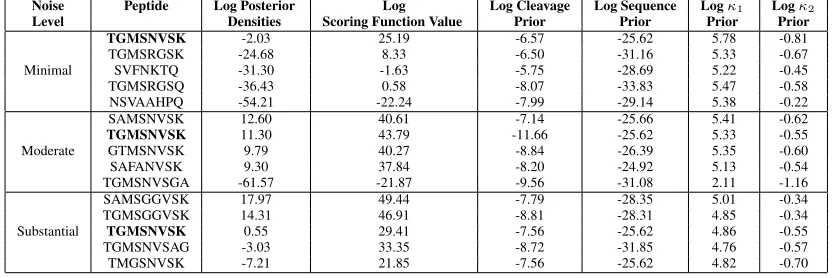
Table 1 shows the posterior mode for theT GM SN V SKexample using the simulated spectrum for each of the three noise levels using a Laplace noise structure. Table 2 shows the posterior mode for theT GM SN V SKexample using the simulated spectrum for each of the three noise levels using a Poisson noise structure. Both tables provide the estimated log posterior densities with the breakdown of the log posterior. The true peptide is highlighted in bold. Both tables show that when using minimal noise, the true peptide is the top estimated peptide, which ensures our method is performing well in both the Laplace and Poisson case. In cases when the spectrum has more noise, our method was still able to identify the true peptide as among the best choices using either noise structure. With moderate noise, the true peptide is estimated as the best peptide under the Laplace noise structure. Under the Poisson noise structure with moderate noise, the true peptide is estimated as the second best peptide, but notice that the log posterior for the best estimate and the log posterior for the true peptide are quite similar. [[Table 1 goes here]] [[Table 2 goes here]]

5.4 Example 2

Here we set the parameters to be the same as in Section 5.3. We now generate a spectrum for a peptide with a longer amino acid sequence. The generated spectrum is based on the peptideY HF EQST V T SQP ARwhose observed spectrum containsm/zvalues that range from235to1634Da. The total number of true peaks iss = 26and so

s1= 3,s2= 20, ands3= 3using boundary section proportions0.1. The total number of true peaks iss= 26and so

s1= 3,s2= 20, ands3= 3. The total number ofm/zvalues in the observed spectrum with intensity values above a threshold isq= 157and soq1= 39,q2= 79, andq3= 39(up to a constant).

As in Example 5.3, we also simulate spectra with minimal and substantial noise. After the spectrum is simulated, we applied our method to the simulated spectrum. The starting peptide isHY F ET DQAT SKP V K, which was obtained from the results from PepNovo when applied to the real data. The algorithm was run for10000iterations.

Table 3 shows the posterior mode for theY HF EQST V T SQP ARexample using the simulated spectrum for each of the three noise levels under a Laplace noise structure, and Table 4 shows the posterior mode for the

Y HF EQST V T SQP ARexample using the simulated spectrum for each of the three noise levels using Poisson noise. Both tables provide the corresponding estimated log posterior densities with the breakdown of the log posterior. The true peptide is highlighted in bold. Table 3 shows when minimal noise is applied, the true peptide again is the top estimated peptide, which shows our method is performing well. When moderate noise is applied, the true peptide is identified as the best estimated peptide. When substantial noise is applied, we see that the true peptide was not identified in the top estimated peptides, because of the additional noise added into the spectrum. Table 4 shows when minimal noise is applied, the true peptide again is the best estimated peptide, confirming that our method is performing adequately well. With moderate noise, the true peptide is estimated as the second best peptide. With substantial noise, the true peptide is among the top estimated peptides. Although the spectrum has more noise, our method was still able to identify the true peptide as being among the best choices in this example. [[Table 3 goes here]] [[Table 4 goes here]]

5.5 Comparison of Noise Structures

With moderate noise, our method performed equally well under both noise structures for peptides with both short and long amino acid sequences. With minimal noise, once again our method performed equally well under both noise structures for peptides with short and long amino acid structures. With minimal noise, the true peptide was identified in all cases.

(13)

Unlike a discriminative model, a generative model allows one to generate samples from the joint distribution. Genera-tive models are more flexible since they are full probabilistic models of all variables and can be used to simulate values of any variable in the model (Singla and Domingos, 2005). Note our function in Equation 1 used is an approximation to the Laplace model.

6 Real Data Application

Most peptides in the PNNL dataset described in Section 1 are of length 8 to 20 amino acids. Our data include some relatively longer peptides due to the type of equipment used to process the data. Recall the equipment used was a LTQ Orbitrap mass spectrometer, which is a hybrid machine composed of a linear ion trap mass spectrometer and the Orbitrap mass analyzer that uses a fast Fourier transform algorithm (Yates et al., 2009). The dataset contains 1,206 peptides with lengths ranging from 7 to 31 amino acids and an average length of 15.16. The data are doubly charged and the total mass for each peptide is given. The dataset contains a set of masses and corresponding intensities with an average intensity value of50.7.

We first process the data. We choose to remove the doubly charged parent ion from the dataset. A parent ion is the fragment ion generated in mass spectrometry before the ion is broken apart into further ions. Them/zvalue of the

doubly-charged ion is PK

i=1m(pi) + 1

2 . Therefore, we remove the peak at that m/zvalue. Our proposed method

works for pre-processed data. After extensive numerical experimentation, we found that using the 75th percentile to calculate the constant and moving threshold works well. This means we use the observedm/zvalues in the data that have corresponding observed intensity values above the threshold value inT. We looked at several other threshold values to see which optimized the results. As the threshold is decreased, the estimated peptides become less similar to the true peptide. This happens because as we lower the threshold, more noise enters the observed spectrum and the value ofS2in the likelihood is greatly increased. Therefore, our algorithm cannot find the true peptide. As the threshold is increased, at a certain point the estimated peptides become less similar to the true peptide. Although there is less noise in the observed spectrum when the threshold is increased, signal peaks may be removed from the observed spectrum with a large threshold. Thus, our algorithm will not be able to correctly to identify the true peptide. Using a threshold of 75% removes many noisy peaks while still retaining the signal peaks. Tables 7.17 - 7.20 in Lewis (2013) illustrate these results.

The mass spectrometer is not always accurate and this can cause the ion fragments that are detected to be slightly shifted from their theoretical position. Therefore, we use a tolerance level of 0.5 Da. That is, we allow the ion peak locations to be up to±0.5Da from their theoretical positions. We set the initial components ofβandγto be

pb1= 0.05andpy₁ = 0.10. We set these probabilities low because the mass spectrometer rarely captures the firstb andyion. Table 1 in Danˇc´ık et al. (1999) provides prior probabilites for observing aboryion based on experimental spectra. We used those prior probabilities as initial starting values forpbiandpy i. After varying the values ofpbiand

p_{y i}based on extensive experimentation, settingpbiandpy ito equal 0.80 worked well. Therefore, we set all otherpbi andp_{y i}to equal 0.80 fori= 2, . . . , p.

We must also specify the hyperparameters, the most critical, in the Gamma prior distribution forκ1 andκ2. After extensive numerical experimentation, the values ofa1,b1,a2, andb2were set to be 5.5, 0.1, 3, and 100, respectively. From further experimentation, the large temperature parameter was set to 500 and the small temperature parameter is 1. We believe these values work well for the peptides of moderate size peptides studied in this paper. For extremely large peptides, the values of the hyperparameters may need to be adjusted to higher values. Based on experimenta-tion, a general criterion for large peptides (i.e., comprising roughly 30 or more amino acids) is to use values for the hyperparameters that are 5 times larger than those used for moderately sized peptides.

Different tolerances affect the performance of the method. Using a small tolerance like 0.1 Da hardly allows for any error in the mass spectrometer, so that the observed spectrum would need to be aligned almost perfectly with the theoretical spectrum. A large tolerance like 1.0 Da would allow more room for error but it would expand the parameter space that needs to be searched, which could prevent the algorithm from finding the true peptide in an efficient manner.

(14)

number of iterations increases the running time of estimating the peptide. Thus, the results from PepNovo should be used to obtain a starting peptide. We then refine the estimated peptide using our proposed method.

6.1 Example 3

Figure 5 is a plot of the observed spectrum for the peptideT GM SN V SK. The theoretical spectrum aligns nicely with the observed spectrum, although there is quite a bit of noise in the center of the graph even after thresholding. [[Figure 5 goes here]]

Using the results from PepNovo, we obtain a starting peptide, T GF AGGV SGA, which has a total mass that is within 0.5 Da of the weight of the true peptide. After 100,000 iterations, our best estimate for the true peptide is

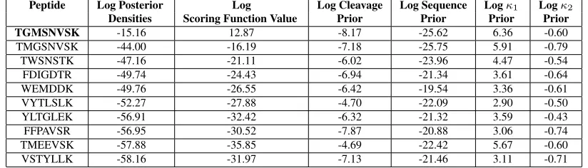
T GM SN V SKwith a log posterior density of−15.16(up to a constant). Table 5 shows the top estimated peptides for theT GM SN V SKexample, with their corresponding estimated log posterior densities and the breakdown of the log posterior (log of the scoring function valueand log priors). The true peptide is estimated as the best having the largest log posterior density. [[Table 5 goes here]]

To ensure our method is obtaining similar results for various starting peptides, consider results from using different starting peptides that we obtain from PepNovo:SAM Y HSK,T GAF GRSK, andGT F AN EGK. Table 6 shows the top estimated peptides along with their corresponding log posterior densities for the above starting peptide values. The results are similar and that the true peptide (highlighted in bold in the table) is captured as the best estimated peptide in all three cases. The log posterior densities are also similar in the three cases. [[Table 6 goes here]]

6.2 Example 4

Figure 6 is a plot of the observed spectrum for the peptide DLV ESAP AALK. The theoretical spectrum aligns nicely with the observed spectrum. [[Figure 6 goes here]]

Using an initial peptide ofDLV ESY F LKfrom the PepNovo results and 100,000 iterations, we obtain our estimate

DLV ESAP AALKwith a log posterior density of42.90(up to a constant). We see that the true peptide is estimated as the best. Table 7 shows the top estimated peptides for theDLV ESAP AALKexample along with the breakdown of the log posterior. [[Table 7 goes here]]

Consider the results from using different starting peptides that we obtain from PepNovo:DLV T DAP AAIQ,

LDV T DAP AALK, andLDV ET GP AAIQ. Table 8 shows the top estimated peptides along with their correspond-ing log posterior densities for the above startcorrespond-ing peptide values. Again the true peptide (highlighted in bold in the table) is the best or is among the best choices in each case, and the log posterior densities are also similar in the three cases. [[Table 8 goes here]]

6.3 Result Comparisons

To quantify objectively how our method improves relative to its current estimation, we compare our results with those using the PepNovo rank score and the PepNovo score. The comparison is only made in the accuracy of the predicted peptide and not in the speed of the computation. Since our method can identify peptides that are not found in a peptide database, we make no comparisons with SEQUEST and MACSOT. We will not make a distinction between the amino acidsIandLbecause they have identical masses of113.084. Although PepNovo does not make a distinction between the amino acidsKandQbecause the difference in their masses is only a minute difference of0.04Da, we will make the distinction.

Our comparison method uses the minimum number of switches in the amino acid sequence of the peptide needed to obtain the true peptide. Switches are only considered if the total mass remains within0.5 Da of the total mass of the true peptide. If the best estimated peptide is the truth, then minimum number of switches would be zero. To illustrate this comparison method, consider the true peptideV SEGQT V Rwith the estimateW EGQT V R. One can see the only difference from the true peptide is that the estimate begins withW while the true peptide begins with

(15)

of permissible switches is1. If more than3switches are needed to obtain the true peptide, we denote the minimum number of switches as 4+. In both the PepNovo rank score and PepNovo score, the best estimated peptide might not have the same mass as the true peptide. PepNovo does provide theN −Gap, which is the mass gap from the N-terminal to the start of the de novo sequence and theC−Gap, which is the mass gap from the C-terminal to the end of the de novo sequence. While it does provide those mass values, it does not detect the amino acid residues that should correspond to the mass gaps. For example, consider the true peptideDLV ESAP AALK with a total mass of1113.616Da. Using the PepNovo rank score, the best estimated peptide isDN V ESLEV, which has a mass of

885.4088Da. Note that this mass is the sum of masses of each amino acid residue in the sequence and does not include the mass of a water molecule and hydrogen molecule. That is accounted for in the mass gap. TheC−Gapvalue given is229.029Da implying there are amino acid residues missing from the end of the de novo sequence whose mass should total229.029Da. We cannot look at the minimum number of switches; however, we do know that a peptide with a total mass less than the total mass (outside of the tolerance) of the true protein cannot be the true peptide.

Table 9 displays the best estimated peptides for the PepNovo rank score, the PepNovo score, and our method along with the corresponding true peptide. The minimum number of switches is in parentheses. One can see that in most cases when using the PepNovo rank score, the best estimated peptide does not have the correct total mass. Thus, refining the results of PepNovo, our method allows our estimated peptides to have the correct total mass (within a tolerance). Comparing the results from the PepNovo score and our method of using the Bayes log posterior, the PepNovo score tends to do slightly better for peptides with shorter amino acid sequences. However, for peptides with longer amino acid sequences, our method tends to do better. PepNovo produces very quick (seconds) results but the MCMC algorithm is slower (several minutes). However, we do not see our method as a competitor but more as a refinement. Note that one method does not necessarily work best in every case, yet a combination of two good methods can produce an even better method. Therefore, an avenue to explore in the future is developing a rank score method that will combine our method with PepNovo’s method. It would be interesting to compare the number of switches for peptides in order to gauge both the false positive and false negative error rates, although this is an enormous computation. [[Table 9 goes here]]

7 Discussion

Proteomics produces large amounts of spectra from mass spectrometry. Issues such as post-translational modifica-tions (PTMs), mutamodifica-tions, and contaminants can cause the spectra to fail to match peptides from a database. Also, there are copious microorganisms such as bacteria and protists that have not been identified and therefore, using a database search to identify these peptides is of very limited use in the case of non-homologous proteins. Of those microorganisms that have been identified, some show evidence of PTMs, which can create complications in the de novo sequencing when comparisons are made between the theoretical spectrum and the observed spectrum. Thus the need for a method of identifying peptides that does not rely on a known database and is not is affected by PTMs is evident.

Another reason for the need for accurate peptide identification is protein sequencing, the method of identifying the true amino acid sequence of a protein. Identifying an entire protein is almost impossible, and so the protein is split into short peptides. Ergo, being able to correctly identify the amino acid sequence of a peptide will aid in identifying the true protein sequencing.

(16)

Cleveland and Rose (2012) developed a method to identify better peaks using a neural network, which can be used to construct a predictive model that does not require an extensive understanding of peptide fragmentation. Like our method, Cleveland and Rose (2012) concentrate on identifying signal peaks corresponding tobandyions; they also employ a leveraged neural network (LNN), which is composed of two neural networks used in order to classify peaks. In the first neural network, peak features, such as isotopologues and neutral losses, are found from the data in the spectrum. Then in the second neural network, the results from the first neural network are leveraged as extra features in the second neural network. This process selects peaks with higher precision and reduces the number of peaks in the spectrum, which could make identifying the true peptide more efficient. Recall from Section 2 that other ions can produce peaks in the observed spectrum. Therefore, employing this method could lead to better identification of peaks, and thus will lead to a more accurate theoretical spectrum and ultimately better identification of peptides. For additional information about the LNN, see Cleveland and Rose (2012).

An important aspect for the future development is to refine the Bayesian model. The model can be refined by including more signal peaks: b−H2O, b−N H3, y−H2O, y−N H3, y2, isotopic peaks, etc, which could aid in identifying which are signal peaks and which are noise peaks. Adapting the prior to assign probabilities to the length of the peptide is another avenue one could explore. The current prior favors shorter peptide sequences. Peptides with shorter amino acid sequences have higher prior probabilities than peptides with longer amino acid sequences.

There are a few other possibilities for future work: Exploration of the sequence prior distribution could be conducted, although a full exploration would be a massive undertaking since the number of sequences is so vast. The calculated priors could be compared with the observed frequencies to gain an idea of how closely the prior distribution reflects the empirical distribution. A sensitivity analysis in the simulations could be explored. Possible approaches to sensitivity analyses would be using a different linear transformation in the cleavage prior, and usingπ(η_F)orπ(η_R)rather than

π(η)in the sequence prior, and seeing whether the results changed much.

Our method is a promising addition to the peptide identification methodological toolbox.

References

Andrieu, C., de Freitas, N., Doucet, A., and Jordan, M. (2003). An introduction to MCMC for machine learning.

Machine Learning, 50(1):5–43.

Ansong, C., Toli´c, N., Purvine, S., Porwollik, S., Jones, M., Yoon, H., Payne, S., Martin, J., Burnet, M., Monroe, M., Venepally, P., Smith, R., Peterson, S., Heffron, F., McClelland, M., and Adkins, J. (2011). Experimental annotation of post-translational features and translated coding regions in the pathogen salmonella typhimurium.

BMC Genomics, 12(1):433.

Bissiri, P. G., Holmes, C. C., and Walker, S. G. (2016). A general framework for updating belief distributions.Journal

of the Royal Statistical Society Series B, 78(5):1103–1130.

Cleveland, J. P. and Rose, J. R. (2012). A neural network approach to the identification of b-/y-ions in MS/MS spectra.

012 IEEE International Conference on Bioinformatics and Biomedicine, 0:1–5.

Coombes, K. R., Baggerly, K. A., and Morris, J. S. (2007). Pre-processing mass spectrometry data. In Dubitzky, M. Granzow, M. and Berrar, D., editors,Fundamentals of Data Mining in Genomics and Proteomics, pages 79–99. Boston: Kluwer.

Damsleth, E. and El-Shaarawi, A. (1989). ARMA models with double-exponentially distributed noise. Journal of the

Royal Statistical Society Series B, 51(1):61–69.

Danˇc´ık, V., Addona, T. A., Clauser, K. R., and Vath, J. E. (1999). De novo peptide sequencing via tandem mass spectrometry: A graph-theoretical approach. In RECOMB ’99: Proceedings of the third annual international

conference on Computational molecular biology, number 135–144, New York, NY, USA. ACM Press.

(17)

Du, P., Stolovitzky, G., Horvatovich, P., Bischoff, R., Lim, J., and Suits, F. (2008). A noise model for mass spectrom-etry based proteomics.Bioinformatics, 24(8):1070–1077.

Frank, A. (2009). A ranking-based scoring function for peptide-spectrum matches. Journal of Proteome Research, 8(5):2241–2252.

Frank, A. and Pevzner, P. (2005). PepNovo: de novo peptide sequencing via probabilistic network modeling.

Analyti-cal Chemistry, 77(4):964–973.

Huang, Y., Triscari, J. M., Pasa-Tolic, L., Anderson, A. G., Lipton, M. S., Smith, R. D., and Wysocki, V. H. (2004). Dissociation behavior of doubly-charged tryptic peptides: Correlation of gas-phase cleavage abundance with ra-machandran plots.Journal of American Chemical Society, 126:3034–3035.

IUBMB(1992). International Union of Biochemistry and Molecular Biology. In Li´ebecq, C., editor, Biochemical

nomenclature and related documents. Portland Press, London. Second Edition.

Kemp, F. (2003). The Laplace distribution and generalizations: a revisit with applications to communications, eco-nomics, engineering, and finance.Journal of the Royal Statistical Society. Series D, 52(4):698–699.

Kirkpatrick, S., Gelatt, C. D., and Vecchi, M. P. (1983). Optimization by simulated annealing.Science, 220(4598):671– 680.

Lewis, C. N. (2013). Protein Identification Using Bayesian Stochastic Search. PhD thesis, University of South Carolina, Retrieved from http://scholarcommons.sc.edu/etd/2674.

Lubec, G. and Afjehi-Sadat, L. (2007). Limitations and pitfalls in protein identification by mass spectrometry.

Chem-ical Reviews, 107(8):3568–3584.

Ma, B., Zhang, K., Hendrie, C., Liang, C., Li, M., Doherty-Kirby, A., and Lajoie, G. (2003). PEAKS: Powerful soft-ware for peptide de novo sequencing by tandem mass spectrometry.Rapid Communications in Mass Spectrometry, 17:2337–2341.

Robert, C. P. and Casella, G. (1999). Monte Carlo Statistical Methods. Springer-Verlag.

Rose, J. R., Cleveland, J. P., and Fox, A. (2010). An information theoretic approach to rescoring peptides produced by de novo peptide sequencing. International Conference on Bioinformatics and Computational Biology (Paris,

France), World Academy of Science, Engineering and Technology, pages 200–205.

Schulze, W. (2004). Environmental proteomics - what proteins from soil and surface water can tell us: a perspective.

Biogeosciences Discussions, 1:195–218.

Singla, P. and Domingos, P. (2005). Discriminative training of Markov logic networks. Proceedings of the 20th

National Conference on Artificial Intelligence (AAAI), pages 868–873.

Sorensen, D. and Gianola, D. (2002). Likelihood, Bayesian and MCMC methods in quantitative genetics. Springer, New York.

Tierney, L. (1994). Markov chains for exploring posterior distributions. The Annals of Statistics, 22(4):1701–1728.

Visintin, I., Feng, Z., Longton, G., Ward, D. C., Alvero, A. B., Lai, Y., Tenthorey, J., Leiser, A., Flores-Saaib, R., Yu, H., Azori, M., Rutherford, T., Schwartz, P. E., and Mor, G. (2008). Diagnostic markers for early detection of ovarian cancer.Clinical Cancer Research, 14:1065–1072.

Wulfkuhle, J. D., Liotta, L. A., and Petricoin, E. F. (2003). Early detection: Proteomic applications for the early detection of cancer. Nature Reviews Cancer, 3:267–275.

Xu, C. and Ma, B. (2006). Software for computational peptide identification from MS-MS data. Drug Discovery

Today, 11(13-14):595–600.

(18)

[image:18.612.88.526.108.254.2]

Table 1: The top estimated peptides from the MCMC algorithm along with their corresponding log posterior densities, log of the scoring function value, log cleavage prior, log sequence prior, logκ1prior, and logκ2prior for the peptide

T GM SN V SKwhen using a simulated spectrum for each of the three noise levels using a Laplace noise structure. Noise Peptide Log Posterior Log Log Cleavage Log Sequence Logκ1 Logκ2

Level Densities Scoring Function Value Prior Prior Prior Prior

Minimal

TGMSNVSK -42.58 -12.84 -8.03 -25.62 5.30 -1.40

TGMYHSK -47.51 -20.86 -7.51 -22.00 4.37 -1.51

FADTIEK -49.95 -25.52 -6.41 -20.21 3.35 -1.15

WIFSDR -50.66 -28.08 -4.84 -20.35 3.82 -1.20

FVNNSDK -54.76 -26.37 -6.98 -22.18 2.15 -1.39

Moderate

TGMSNVSK -27.82 0.98 -8.94 -25.62 6.08 -0.32

AEPTDYK -47.97 -24.68 -5.39 -21.15 3.76 -0.50

DEMLTSK -49.36 -24.43 -5.85 -22.76 4.17 -0.49

ASAYQQR -49.39 -22.53 -8.26 -21.49 3.37 -0.48

APNLAIPK -51.56 -22.29 -8.97 -22.70 2.94 -0.54

Substantial

TGMPFDR 27.89 47.60 -4.20 -21.79 5.94 0.34

TGMSNVTGG 26.22 63.06 -11.25 -31.85 6.00 0.25

TTSSNVASG 16.59 49.34 -7.83 -31.11 6.00 0.19

TGMSNVSQ 14.27 41.50 -5.23 -28.29 6.04 0.25

TGMSNVSK 7.23 37.53 -10.95 -25.62 6.06 0.21

T GM SN V SKwhen using a simulated spectrum for each of the three noise levels using a Poisson noise structure. Noise Peptide Log Posterior Log Log Cleavage Log Sequence Logκ1 Logκ2

Minimal

TGMSNVSK -2.03 25.19 -6.57 -25.62 5.78 -0.81

TGMSRGSK -24.68 8.33 -6.50 -31.16 5.33 -0.67

SVFNKTQ -31.30 -1.63 -5.75 -28.69 5.22 -0.45

TGMSRGSQ -36.43 0.58 -8.07 -33.83 5.47 -0.58

NSVAAHPQ -54.21 -22.24 -7.99 -29.14 5.38 -0.22

Moderate

SAMSNVSK 12.60 40.61 -7.14 -25.66 5.41 -0.62

TGMSNVSK 11.30 43.79 -11.66 -25.62 5.33 -0.55

GTMSNVSK 9.79 40.27 -8.84 -26.39 5.35 -0.60

SAFANVSK 9.30 37.84 -8.20 -24.92 5.13 -0.54

TGMSNVSGA -61.57 -21.87 -9.56 -31.08 2.11 -1.16

Substantial

SAMSGGVSK 17.97 49.44 -7.79 -28.35 5.01 -0.34

TGMSGGVSK 14.31 46.91 -8.81 -28.31 4.85 -0.34

TGMSNVSK 0.55 29.41 -7.56 -25.62 4.86 -0.55

TGMSNVSAG -3.03 33.35 -8.72 -31.85 4.76 -0.57

[image:18.612.97.513.316.455.2]

(19)

[image:19.612.76.529.130.281.2]

Y HF EQST V T SQP ARwhen using a simulated spectrum for each of the three noise levels using a Laplace noise structure.

Noise Peptide Log Posterior Log Log Cleavage Log Sequence Logκ1 Logκ2

Minimal

YHFEQSTVTSQPAR 6.21 55.98 -10.29 -47.30 5.99 0.22

YHFSEGSSVVSQPAR 4.40 62.07 -16.64 -47.08 5.86 0.19

YHFSEKTVTSQPAR 3.60 55.12 -10.29 -47.30 5.82 0.25

YHFSEGATTVSQPAR 2.45 60.22 -16.64 -47.08 5.79 0.16

LIAFFNGGGATCHEVD -41.45 29.23 -16.33 -59.10 4.72 0.04

Moderate

YHFEQSTVTSQPAR 88.52 141.08 -13.57 -44.63 5.44 0.19

YHFEQSTVTNTPVQ 86.87 145.87 -17.28 -47.56 5.67 0.16

GDKFEQSTVTSQPAR 85.00 147.05 -18.65 -49.15 5.62 0.14

YHFEQSTVTNTPAR 84.01 134.36 -12.12 -43.85 5.53 0.09

YHFAWSTVTSQPAR 41.81 102.71 -18.84 -46.80 4.63 0.11

Substantial

YHFEQSTVTQSPLN 180.51 241.92 -18.71 -49.14 5.75 0.68

YHFEKSTVTQSPAR 163.42 220.25 -14.52 -48.20 5.16 0.73

YHFEKSTVTSKPAR 157.52 218.14 -16.35 -50.41 5.45 0.69

YHFEQSTVTQSPAR 154.39 206.48 -13.09 -44.69 5.02 0.67

[image:19.612.76.531.364.505.2]

YHFEQSTSISQPAR 116.96 169.27 -12.00 -45.25 4.39 0.55

Y HF EQST V T SQP ARwhen using a simulated spectrum for each of the three noise levels using a Poisson noise structure.

Noise Peptide Log Posterior Log Log Cleavage Log Sequence Logκ1 Logκ2

Minimal

YHFEQSTVTSQPAR 48.16 101.54 -14.20 -44.63 4.96 0.49

YHFEQSTVTSKPAR 44.39 100.61 -14.65 -46.89 4.88 0.44

YHFEQSTVTSKPNL 41.20 103.98 -16.84 -50.91 4.55 0.41

YHFEQSTPCSPAGAR -9.05 58.66 -14.34 -58.55 4.78 0.39

YHFEKSPTSSSGPAR -68.16 0.13 -15.63 -57.43 4.33 0.45

Moderate

YHFQTFAVEGQPAVG 8.55 74.36 -17.51 -52.15 3.76 0.10

YHFEQSTVTSQPAR 6.41 77.81 -20.77 -54.41 3.67 0.10

YHFGATMEGEGQPAVG -3.28 67.19 -20.01 -53.99 3.40 0.11

YHFGAGMETEGQPAVG -9.41 59.44 -18.46 -53.92 3.48 0.05

YHFGATFAVEGQPAVG -47.16 18.95 -20.45 -48.14 2.67 -0.17

Substantial

YHFEQSTVTSGAPAR 140.22 192.03 -17.16 -47.31 5.92 0.40

YHFEAGSTVTSGAPAR 135.46 190.34 -17.10 -49.72 5.58 0.41

YHFEAGSTVTSKPAR 133.49 183.83 -13.50 -49.31 5.87 0.36

YHFEQSTVTSQPAR 128.28 173.90 -13.44 -44.63 5.86 0.37

[image:19.612.99.511.588.706.2]

YHFEQSTVMGQPAR 116.28 165.56 -15.99 -45.28 5.66 0.33

T GM SN V SK. The true peptide is in bold.

Peptide Log Posterior Log Log Cleavage Log Sequence Logκ1 Logκ2

Densities Scoring Function Value Prior Prior Prior Prior

TGMSNVSK -15.16 12.87 -8.17 -25.62 6.36 -0.60

TMGSNVSK -44.00 -16.19 -7.18 -25.75 5.91 -0.79

TWSNSTK -47.16 -21.11 -6.02 -23.96 4.47 -0.54

FDIGDTR -49.74 -24.43 -6.94 -21.34 3.61 -0.64

WEMDDK -49.76 -26.55 -6.42 -19.54 3.36 -0.61

VYTLSLK -52.27 -27.88 -4.70 -22.09 2.90 -0.50

YLTGLEK -56.91 -32.42 -6.32 -21.32 3.59 -0.43

FFPAVSR -56.95 -30.52 -7.87 -20.88 3.06 -0.74

TMEEVSK -57.88 -35.85 -4.69 -22.42 5.67 -0.60

(20)

[image:20.612.130.483.139.265.2]

Table 6: The top estimated peptides from the MCMC algorithm along with their corresponding log posterior densities for the peptideT GM SN V SKfor three different starting peptides. The true peptide is in bold.

Starting Peptide

SAMYHSK TGAFGRSK GTFANEGK

Peptide Log Posterior Peptide Log Posterior Peptide Log Posterior

TGMSNVSK -14.31 TGMSNVSK -17.95 TGMSNVSK -14.67

SMTQTQK -49.50 ITLYADK -27.54 MGSNVSQ -22.76

TMTLETQ -50.12 TGMVTTTL -31.73 TFQSQWK -36.20

SLSIYLK -52.39 MGAITMSI -41.43 VMDPFSK -40.15

GYDNLNK -54.01 CGMEAANK -44.11 AYIISEK -41.73

EATFDLK -55.05 FLVDAMK -44.76 YGPETEK -47.05

HFPIPGR -55.601 TGMSDVLT -51.78 TWYVVR -48.64

YDQPATE -56.13 FFGLIAR -51.88 DVFDSLK -48.89

GAQYGEAK -57.43 TGMSLTTL -52.84 WHLPDR -49.39

[image:20.612.93.493.379.478.2]

WTYLLQ -58.16 -ITLYVSK -52.10 TGAFNWK -57.68

DLV ESAP AALK.

Peptide Log Posterior Log Log Cleavage Log Sequence Logκ1 Logκ2

Densities Scoring Function Value Prior Prior Prior Prior DLVESAPAALK 42.90 78.94 -11.25 -31.26 6.31 0.15

AVQIEQVQAQ 8.56 47.48 -8.57 -33.83 3.51 -0.03

DLVESPAAAIK 2.63 40.03 -11.28 -31.69 5.435 0.14

LTELASPAALQ -0.94 38.74 -10.70 -34.13 4.92 0.23

DLVESAPAAIK -1.65 35.86 -11.28 -31.69 5.38 0.07

QVDIVLGDVR -7.24 30.33 -11.50 -29.70 3.42 0.21

QVDIIVDGVR -14.54 23.36 -12.99 -29.67 4.61 0.16

EVPATTGGVGPE -16.30 29.28 -12.53 -37.61 4.52 0.04

QVDIPDDGVR -16.89 21.68 -12.99 -29.67 4.15 -0.04

EVPTATGGVGPE -17.22 27.76 -12.53 -37.61 4.89 0.27

Table 8: The top estimated peptides from the MCMC algorithm along with their corresponding log posterior densities for the peptideDLV ESAP AALKfor three different starting peptides. The true peptide is in bold.

Starting Peptide

DLVTDAPAAIQ LDVEYYALK LDVETGPAALK

Peptide Log Posterior Peptide Log Posterior Peptide Log Posterior

DDLTVAAPAIK 30.35 DLVESAPAALK 31.51 DLVDTAAPALK 35.76

DLVESAPAALK 21.05 VADPANGQLTQ 11.97 DLVESAPAALK 29.99

AVSPAWGNLAK 14.49 SPFSISYANK -5.26 LDVDVAGAPEK 7.25

MVIVTAAPLAK 3.01 DQSNDYDEK -8.41 LDVTIAGAPEK -5.06

DLTPVSVSPAK -1.97 DLVESAPIAAK -8.81 APVDIIQDDK -7.49

DDLLGTAPALK -4.03 DAEDMYLK -9.49 DLVDTAPAALK -9.00

NNVEASPAALK -5.12 ELEGNEPMPVK -9.64 MDMMEDLTK -15.49

DPVDWVAALK -6.57 VFPLSPDNPK -16.21 DLLTTAPAALK -19.25

DDLVTAAPAIK -15.07 DVLASEPASPK -23.99 DLLATTPAALK -20.61