Forecast evaluation tests and negative long run variance estimates in small samples

Forecast Evaluation Tests and Negative Long-run

Variance Estimates in Small Samples

David I. Harvey, Stephen J. Leybourne and Emily J. Whitehouse

School of Economics, University of Nottingham

May 3, 2017

Abstract

In this paper, we show that when computing standard Diebold-Mariano-type tests for equal forecast accuracy and forecast encompassing, the long-run variance can frequently be neg-ative when dealing with multi-step-ahead predictions in small, but empirically relevant, sample sizes. We subsequently consider a number of alternative approaches to dealing with this problem, including direct inference in the problem cases and use of long-run variance estimators that guarantee positivity. The …nite sample size and power of the di¤erent approaches are evaluated using extensive Monte Carlo simulation exercises. Overall, for multi-step-ahead forecasts, we …nd that the recently proposed Coroneo and Iacone (2016) test, which is based on a weighted periodogram long-run variance estimator, o¤ers the best …nite sample size and power performance.

Keywords: Forecast evaluation; Long-run variance estimation; Simulation; Diebold-Mariano test; Forecasting.

JEL Classi…cation: C12, C22, C53.

1

Introduction

Given the critical role that forecasting plays in economic and …nancial research and

policy-making, the evaluation of competing forecasts of the same outcomes has become an extensive

and prominent …eld in the econometric and empirical economic literatures. Within this …eld,

the most common forecast evaluation exercise typically undertaken is to compare the accuracy

of two or more sets of forecasts on the basis of some measure of loss associated with the forecast

errors, such as mean squared forecast error. In a key contribution to the literature, Diebold

and Mariano (1995) [DM] proposed an approach for testing equal forecast accuracy valid for

potentially contemporaneously correlated, serially correlated and non-normal forecast errors,

based on testing for a zero mean in a series de…ned as the di¤erence between the two forecasts’

error loss functions (the “loss di¤erential”). Harvey et al. (1997) [HLNa] suggested two …nite

sample modi…cations to the DM statistic to improve size control in small samples, based on a

…nite sample bias correction to the test statistic, and using Student’s t critical values rather

than those from a standard normal. Application of the DM test or its HLNa variant have now

become prevalent in empirical forecasting research, to the extent that it is now routine for the

results of such forecast accuracy tests to be reported alongside any forecast comparisons.

Testing for equal forecast accuracy is just one approach to evaluating the predictive ability

of rival forecasts. A second popular evaluation method is to test for whether one set of forecasts

encompasses another, in the sense that the encompassed forecasts do not result in a reduction in

forecast accuracy when used in combination with the encompassing set of forecasts. Harveyet

al. (1998) [HLNb] proposed a forecast encompassing test based on a DM-type approach, where

the loss di¤erential is rede…ned to permit testing an encompassing null hypothesis, and the

approach has become standard in cases where one abstracts from model parameter estimation

uncertainty.

In this paper we focus on the behaviour of the DM/HLNa tests based on squared error loss,

and the HLNb test for encompassing, in small samples. Our work is therefore in a similar vein

to that of Ashley (2003) and Ashley and Tsang (2014) who investigate out-of-sample inference

with limited data availability. The DM test statistic is fundamentally comprised of the loss

di¤erential series sample mean standardised by an estimate of the long-run variance. DM make

use of the fact that optimal h-steps-ahead forecasts are at most (h 1)-order dependent to

advocate use of a rectangular kernel in the long-run variance estimator which truncates at lag

h 1. While this approach results in decent …nite sample size and power properties for many

sample size and h settings, the long-run variance estimator is not guaranteed to be positive whenever h > 1. DM note this possibility, but suggest that such an outcome would be rare; similarly, Clark (1999) …nds a low occurrence of negative long-run variance estimates in his equal

accuracy test simulations (always less than 3% of replications). However, these observations

were made on the basis of results that considered predictions only up to two steps ahead. Our

be much greater in small samples when longer horizon forecasts are considered. For example,

when testing equal mean squared forecast error with h = 6, we …nd that negative variance

estimates arise approximately 20% of the time for a sample size of 16, rising to over 40% of the

time for a sample size of 8.

In practical applications, often due to the limitations of economic or forecast data, it is

not uncommon for forecast evaluation to be conducted using sample size and forecast horizon

settings that lie in the region where negative variance estimates occur frequently. For example,

in the context of testing for equal forecast accuracy, the recent papers Caporale and Gil-Alana

(2014), Dreger and Wolters (2014), Dib et al. (2008) and Qin et al. (2008) all implement

the DM/HLNa tests in forecast samples smaller than 25 observations with horizons of h = 6 or greater. Further, Mehl (2009) and Chow and Choy (2006) have reported …nding negative

DM/HLNa long-run variance estimates when using samples of 18 and 24 forecasts at horizons

of 6 and 5-6, respectively.

Given that negative variance estimates can arise frequently in situations of practical

rele-vance, it is important to determine the best approach to deliver a reliable testing procedure

in terms of small sample size and power properties. DM suggest treating a negative variance

estimate as a zero, thereby automatically rejecting the null against a two-sided alternative in

such cases. However, given the low occurrence of negative variance estimates in their

simula-tions, the size implications of such an approach are not fully explored. In the simulation work

of Clark (1999), the relatively few replications where negative variance estimates were obtained

were excluded from the simulations, thereby abstracting from the e¤ects of dealing with certain

problematic cases. HLNa and HLNb simulated combinations of sample size and forecast

hori-zon where negative variances can occur frequently, but their simulations failed to correctly deal

with negative variance estimates, thus again the impact of negativity in the variance estimate

is not clear. Of course, other long-run variance estimators exist which ensure non-negativity;

for example, DM, Clark (1999) and others discuss the possible use of the Bartlett kernel, and

in a recent paper on testing equal forecast accuracy, Coroneo and Iacone (2016) recommend

use of the nonparametric periodogram estimator of Hualde and Iacone (2017), combined with

use of bandwidth-dependent critical values. The second contribution of this paper is therefore

to formally assess the behaviour of di¤erent strategies for dealing with the potential problem of

negative long-run variance estimation in tests of equal accuracy and encompassing. We conduct

an extensive set of Monte Carlo simulations to establish the small sample size and power

prop-erties of di¤erent approaches. Broadly, we …nd that for multi-step-ahead forecasts, the Coroneo

and Iacone (2016) approach outperforms other methods, and the attractive …nite sample

prop-erties reported in their paper for moderate sample sizes and forecast horizons extends to the

small sample and longer horizon region under focus in this paper for both equal accuracy and

encompassing tests, where the DM/HLNa and HLNb tests can su¤er from negative variance

estimates.

and HLNb tests for equal mean squared forecast error and forecast encompassing. Section 3

highlights by simulation the frequency with which negative long-run variance estimates can

arise for di¤erent sample sizes and forecast horizons. In section 4, a number of ways of dealing

with these cases are considered, including alternative long-run variance estimators that are

guaranteed to be positive, and section 5 investigates the performance of these procedures using

…nite sample size and power simulations. In section 6 we conduct a related set of simulation

experiments using a DGP calibrated to the empirical work of Dreger and Wolters (2014), while

section 7 considers simulations for the case where forecasts are obtained from estimated models.

Section 8 concludes.

2

Standard tests for equal accuracy and encompassing

Consider …rst the issue of evaluating whether two competing sets of forecasts are equally

accu-rate according to some loss function-based accuracy measure, or whether one forecast

outper-forms the other in terms of that metric. Denote the actuals byyt and the competing forecasts

byf1tand f2t,t= 1; :::; T, and consider a given loss functionL(:) that depends on the forecast

errors, so that the cost of error associated with the forecast fit is L(eit),i= 1;2. Now de…ne

the loss di¤erential series

dt=L(e1t) L(e2t); t= 1; :::; T:

The null hypothesis of equal forecast accuracy, according to the speci…ed loss functionL(:), can

then be expressed as

H0 :E(dt) = 0:

For example, under squared error loss,dt=e21t e22tand the null hypothesis entails the equality

of population mean squared forecast errors.

Under the assumptions that dt is covariance stationary and short memory, DM propose a

test of H0 based on the asymptotic distribution of the sample mean loss di¤erential

p

T(d E(dt)) d

!N 0; !2

where d=T 1PT_t=1dt and !2 denotes the long-run variance of dt, i.e. !2 =P1j= 1 j with j = Cov(dt; dt j). Denoting a consistent long-run variance estimator by !^2, the DM test

statistic is then given by

DM =pT d

^

!

which has an asymptotic standard normal distribution under the null. DM suggest use of

a long-run variance estimator comprised of a weighted sum of sample autocovariances, and,

they advocate using a rectangular kernel truncated at lagh 1, i.e.

^

!2= ^₀+ 2

h 1

X

j=1

^_j (1)

where^_j =T 1PT_t=j+1 dt d dt j d .1 HLNa propose a modi…cation of the DM statistic

designed to improve the small sample size behaviour of the test. Their statistic is based on an

approximate bias correction to the long-run variance estimator, and can be written as

M DM =pT+ 1 2h+T 1_{h(h 1)} d

^

! : (2)

These authors also suggest use oftT 1critical values in place of those from the standard normal,

again to better control small sample size.

Next consider investigating whether one set of forecasts encompasses another, in that the

accuracy of one set of (encompassing) forecasts f1t cannot be improved through linear

com-bination with a second set of (encompassed) forecasts f2t. HLNb develop a test for forecast

encompassing based on the Bates and Granger (1969) forecast combination scheme, where the

combination weights sum to one.2 Denoting the combined forecast by fct, the combination is

fct = (1 )f1t+ f2t

where (0 1) determines the weights associated with the constituent forecasts. In this

context, forecast f1t encompasses forecast f2t if the optimal mean squared error-minimising

combination weight

opt =

E(e2_1t) E(e1te2t)

E(e2

1t) +E(e22t) 2E(e1te2t)

is equal to zero. The null of forecast encompassing can then be expressed in a DM-type form:

H0 :E(dt) = 0

withdt in this case de…ned as

dt=e1t(e1t e2t): (3)

HLNb therefore propose applying the DM approach to this testing problem, along with the

HLNa bias correction and use of tT 1 critical values. The test statistic is then (2) but with dt

given by (3). The test is conducted against the one-sided alternative E(dt) > 0 (i.e. > 0),

given the assumption of a non-negative combination weight.

1

Note that ARCH-type behaviour in the forecast errors induces additional autocorrelation intodt, requiring use of higher order lags; see Harvey, Leybourne and Newbold (1999).

2

3

Frequency of negative long-run variance estimates

The long-run variance estimator (1), based on the rectangular kernel, is not guaranteed to be

positive wheneverh >1. In practice, of course, a negative outcome is highly problematic since the M DM statistic for testing equal accuracy or encompassing cannot be computed. In such

circumstances, a practitioner must then decide how to deal with such a result; suggestions in

the literature include treating the estimate as zero or using an alternative long-run variance

estimator that guarantees positivity. Whatever strategy is followed will have implications for

the size and power of the resulting testing procedure, so it is therefore valuable to quantify

how frequently negative long-run variance estimates are likely to be encountered in practice.

While DM, Clark (1999) and Coroneo and Iacone (2016),inter alios, note that (1) can produce a

negative result, little evidence has so far been provided as to the extent of this potential problem.

To shed more light on the issue, in this section we report results from Monte Carlo simulation

experiments to determine the frequency with which negative long-run variance estimates arise

for di¤erent sample sizes and forecast horizons, both for equal accuracy and encompassing tests.

To begin, we consider the case of testing for equal forecast accuracy, adopting a standard

simulation data generating process [DGP] consistent with the work of DM, HLNa and Clark

(1999). We assume mean squared error loss, so that dt = e21t e22t, t = 1; :::; T, generating

the forecast errors according to the following DGP, which allows forh-steps-ahead forecasts to

follow moving average [MA] processes of orderh 1:

e1t = v1t+ h 1

X

j=1

jv1;t j

e2t =

p

R

0 @v2t+

h 1

X

j=1

jv2;t j

1 A

where[v1t; v2t]0 N(0; I2),t= 1 (h 1); :::; T. The ratio of the variances of the two forecast

errors is given by R > 0, with R = 1 giving the null and R ₆= 1 the alternative. Focusing

on the small samples that are often employed in forecast evaluation exercises, we simulate this

DGP forT =_f8;16;32;64_g,h=_f2;3;4;5;6_g, and calculate the frequency with which negative

values of the long-run variance estimator (1) arise. We consider three settings for the MA

parameters: (i) the case of no serial correlation with j = 0 8j, (ii) a case of moderate serial

correlation with j = 0:9=(h 1) 8j, and (iii) a case of high degree serial correlation with j

set to the jth element of = (0:95;0:9;0:8;0:65;0:6), these values being drawn from the US in‡ation forecast error-based DGP 1 of Clark and McCracken (2013). Here and throughout the

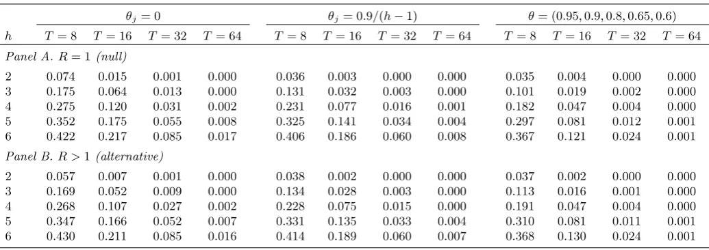
paper, simulations are conducted using 10,000 Monte Carlo replications. Table 1 reports the

results under the null (R = 1), and under the alternative (R >1), with the settings R = 12,

R= 7,R= 3 and R= 2forT = 8,T = 16,T = 32andT = 64, respectively (chosen to ensure that the test powers considered in section 5 are roughly comparable across sample sizes).

that increases with the forecast horizon, and decreases with the sample size. While the

occur-rence of negative estimates is rare whenT = 64, the problem can be substantial for the smaller

sample sizes considered, particularly for longer forecast horizons where the frequency can rise

above 40%. In such circumstances, a practitioner would be unable to compute the standardDM

orM DM test statistics almost half the time. The pattern of frequencies for negative long-run variance estimates has very little dependence on whether the simulations are conducted under

the null or alternative hypotheses, and while there is a reduction in the frequency of negative

estimates as the degree of serial correlation increases, the overall features of the results are

sim-ilar across the di¤erent dependence settings, particularly for the longer forecast horizons. We

also considered simulations where the forecast errors were contemporaneously correlated, but

this had little e¤ect on the proportion of negative long-run variances obtained. These results

highlight a potentially serious issue with the implementation of standard tests for equal forecast

accuracy in small samples.

Turning now to testing for forecast encompassing, we let dt = e1t(e1t e2t), t = 1; :::; T,

where the forecast errors are generated according to the following DGP, again allowing for

MA(h 1)-dependence in the errors ofh-steps-ahead forecasts:

eit=vit+ h 1

X

j=1

jvi;t j; i= 1;2

where _"

v1t

v2t

#

N 0;

"

1

2

#!

; t= 1 (h 1); :::; T

with 2 > 2. The null hypothesis that forecast f1t encompasses f2t is obtained by setting

= 1, while a setting of < 1 gives the alternative. Under the alternative, it can be shown

that power depends only on the single parameterk=p 2 2_{=(1 ). Table 2 reports results}

for the frequency of negative long-run variance estimates using the same settings for T, h and

j as in Table 1. Results are reported under both the null and alternative, with the settings

fork under the alternative beingk= 1:25,k= 2:00,k= 3:00 and k= 4:50 forT = 8,T = 16,

T = 32andT = 64, respectively (again chosen to broadly align the test power levels considered

in section 5 across sample sizes).

The pattern of negative estimates for the long-run variance is very similar in the case of

testing for forecast encompassing to that for testing for equal forecast accuracy. Indeed, on

comparing Tables 1 and 2 for a given combination ofT,h and j, it is clear that the numerical

frequencies are very close to each other, suggesting that the prevalence of negative long-run

variance estimates is driven more by the interplay of sample size, serial correlation and the

number of estimated autocovariances (h 1), rather than by the precise form of dt. We again

see a rising incidence of negative estimates asT decreases and ashincreases. As with the equal accuracy results, it makes little di¤erence whether the long-run variance is being calculated

serial correlation. The overall …nding is that negative long-run variance estimates can occur

with very high probability for equal accuracy and encompassing tests when using

multi-step-ahead forecasts with small, yet practically relevant, sample sizes.

4

Adjusted Diebold-Mariano-type tests

Given the prevalence of negative long-run variance estimates that arise for multi-step-ahead

forecasts in small samples when using the standard long-run variance estimator in the DM-type

tests, it is important to establish methods for dealing with this potential problem. In this

section we consider a number of possible approaches, all based on the DM-type tests for equal

accuracy and encompassing. The following section then evaluates their relative performance in

terms of …nite sample size and power.

The …rst approach we consider is the suggested method of DM in the equal accuracy testing

context, which is to treat any occurrence of a negative long-run variance as a zero, viewing the

negative estimate as indicative of a very small long-run variance. This of course implies a test

statistic of ₁, depending on the sign of the numeratord. In a two-sided testing context, as in DM, such a treatment induces an immediate rejection of the null hypothesis, so a negative

long-run variance estimate always indicates evidence in favour of the alternative hypothesis under

this approach. When testing against a one-sided alternative, as is common in applications of

equal accuracy tests and always the case when testing for encompassing, treating a negative

long-run variance as zero will either induce automatic rejection or non-rejection, depending on

whether the implied test statistic value of +₁ or ₁ lies in the relevant one-tailed critical

region. Applying this approach to the M DM tests of HLNa and HLNb, we can express the method as

M DMrej =

(

M DM if!^2>0

sign(d) ₁ otherwise

with the test statistic to be compared withtT 1 critical values.

Given the frequency with which negative long-run variance estimates can occur, theM DMrej

approach will induce substantial over-size in two-sided equal accuracy testing procedures for

h >1 and smallT, as all occurrences of a negative!^2 trigger a rejection of the null. A similar,

albeit reduced, feature of over-size would also be expected for one-sided equal accuracy tests

and tests for forecast encompassing, with rejections of the null occurring whenever a negative

^

!2 coincides with the appropriate sign ofd. A simple conservative approach which would avoid such properties is to treat the occurrence of a negative long-run variance estimate as a failure

to correctly estimate the true long-run variance, and default tonon-rejection of the null in such

instances. One way of writing such a method would be to de…ne the adjusted test statistic as

M DMnon=

(

M DM if!^2 >0

with the test statistic again being compared with tT 1 critical values. A potential down-side

of this approach is that the greater size control a¤orded by treating negative estimate cases as

non-rejections is also likely to be associated with low power under the respective test alternative.

Another simple approach is to deal with a negative long-run variance estimate by replacing

it with the corresponding short-run variance estimate ^₀, thereby reducing the bandwidth in

(1) from h 1 to zero. While this approach neglects the impact of autocorrelation terms, it can be argued that the very presence of a negative estimate indicates that estimation of such

components is highly unreliable in these situations. When the short-run variance estimator is

used, the appropriate bias correction in the M DM statistic is that forh= 1, i.e.

M DM0 =

p

T 1 pd

^₀

!

and the overall test statistic that adopts this statistic when a negative long-run variance is

encountered can be written as

M DMSR=

(

M DM if!^2 >0

M DM0 otherwise

:

Critical values from the tT 1 distribution are again to be used.

While the above methods replace negative long-run variances with simple decision rules or

a short-run variance estimate, the next two approaches we consider retain a proper estimate of

the long-run variance, but make use of estimators that impose positivity. An obvious possibility

in this class is to replace the rectangular kernel in (1) with the Bartlett kernel, i.e.

^

!2_Bart= ^₀+ 2

m

X

j=1

1 j

m+ 1 ^j

wherem denotes the bandwidth. Clark (1999) considered such an approach with Newey-West

and pre-whitened Newey-West bandwidth selection. While Clark’s simulations abstracted from

issues of negative variance estimation, it was found that a Bartlett-based approach could result

in greater …nite sample over-size than when using the rectangular kernel, hence it would not be

recommended to use the Bartlett kernel in all circumstances, particularly when the rectangular

kernel does not have negative variance estimate problems. Here, we consider a hybrid approach,

whereby the standard M DM test is used provided the long-run variance estimate is positive, but in the case of a negative estimate, the statistic switches to one based on the Bartlett kernel.

For consistency with the optimal forecast-motivated choice of truncation h 1 in (1), along with the fact that use of the Bartlett kernel is most likely to arise in small samples, we set the

Bartlett bandwidth to m =h 1. As the HLNa bias correction does not apply to !^2_Bart (and an equivalent bias correction is not possible to obtain without e¤ectively reducing!^2_Bartto!^2), we de…ne the DM statistic that uses the Bartlett long-run variance estimator as

DMBart=

p

T d

^

!Bart

We can then write the third testing approach as

M DMB=

(

M DM if!^2 >0

DMBart otherwise

withtT 1 critical values employed as before.

The original DM test, and the variants outlined above, all make use of weighted sample

au-tocovariances in the long-run variance estimator. An alternative approach proposed by Coroneo

and Iacone (2016) is to use a weighted periodogram estimator, and these authors recommend

construction of a DM-type test using the estimator of Hualde and Iacone (2017). Denoting the

periodogram ofdtfor Fourier frequency j = 2 j=T by

I( j) =

1 p

2 T

T

X

t=1

dte i jt

2

withithe imaginary unit, they suggest use of the Daniell kernel with bandwidthmto construct the weighted periodogram estimator of the long-run variance

^

!2_Dan = 2 1

m

m

X

j=1

I( j)

which is then used to construct the DM-type test statistic

DMCI =

p

T d

^

!Dan

:

If the bandwidth is treated as …xed, !^2_Dan is not a consistent estimator of !2, but is asymp-totically unbiased, and under the null hypothesis of E(dt) = 0, DMCI follows an asymptotic

t2m distribution. This …xed-m treatment results in a test with appealing …nite sample

prop-erties, o¤ering better size control relative to the m _{! 1} treatment that results in standard normal limit theory. Coroneo and Iacone observe that thet2m distribution can act as a better

approximation of the true null distribution for a smaller bandwidth, whereas larger bandwidths

can be associated with higher power, hence a size-power trade-o¤ emerges. Following these

authors, we consider two versions of the test, setting the bandwidths according to m= T1=3

and m = T1=4 (where _b:_c denotes the integer part of the argument), denoting the resulting test statistics by DMCI;1 and DMCI;2, respectively. Note that for any given sample size, m

is then treated as a …xed number so that the …xed-m asymptotic theory can be applied, with critical values drawn from the t2m distribution.

In addition to the above methods, we also experimented with other possible solutions to the

negative variance estimate problem. We considered replacing a negative long-run variance

esti-mate with a modi…ed estiesti-mate based on reducing the rectangular kernel bandwidth sequentially

until a positive estimate was obtained, and we investigated the exponential covariogram-based

long-run variance estimator proposed in the spatial prediction context by Hering and

bandwidth h 1, examining results for the Bartlett kernel using a larger bandwidth setting of 2(h 1), and also the standard and pre-whitened quadratic spectral long-run variance

estima-tors of Andrews (1991) and Andrews and Monahan (1992) with automatic bandwidth selection.

However, these alternatives did not deliver superior …nite sample size and power performance

relative to the better of the approaches considered above, hence we do not detail these tests

and their results in this paper; full results are available from the authors on request.

5

Finite sample size and power

In this section we consider the …nite sample performance of the di¤erent methods outlined in the

previous section. We …rst consider testing for equal forecast accuracy, again focusing on mean

squared error loss (dt=e21t e22t), and simulate the empirical sizes of the M DMrej,M DMnon,

M DMSR,M DMB,DMCI;1 andDMCI;2 testing approaches, with the tests conducted against

a two-sided alternative at the nominal 0.10-level. In addition to these six approaches, for

comparison we also report results for theDMBart statistic compared withtT 1 critical values,

which always employs the Bartlett kernel-based estimator !^2_Bart regardless of the sign of the rectangular kernel-based estimator !^2. As with the earlier simulations in section 3, we use

a standard simulation setup in line with DM, HLNa and Clark (1999). Table 3 reports the

sizes for the same simulation DGPs that were considered in the negative long-run variance

simulations of section 3 when the null hypothesis was imposed (R= 1). Note thatDMCI;1 and

DMCI;2 are identical when T = 16since T1=3 = T1=4 in this case.

Whenh= 1, the originalM DM statistic cannot su¤er from negative long-run variance

esti-mation problems, soM DMrej,M DMnon,M DMSR,M DMB all amount to simply conducting

M DM. (Note also that when h= 1, no serial correlation is present in the DGP, hence the j

settings play no role.) Here, the test is well behaved, with sizes very close to the nominal level,

with only modest under-size displayed for T = 8 and T = 16. A very similar pattern of size behaviour is also seen for DMCI;1 and DMCI;2, while DMBart exhibits some minor over-size

but is also generally well behaved. All tests are therefore reliable for one-step-ahead forecasts

and there is little to choose between them in terms of …nite sample size.

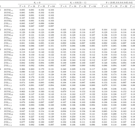
For multi-step-ahead forecasts (h > 1), the possibility of negative long-run variance esti-mates arises and so the method of dealing with these problem cases results in di¤erent size

properties for the overall procedures that we consider. The M DMrej approach translates any

negative long-run variance estimate into a rejection of the null, thus the high frequency of

neg-ative estimates for larger h and smallerT induces a high degree of over-size for this approach.

In line with the results of Table 1, the size of M DMrej reaches almost 0.50, and such large

upward size distortions render this procedure invalid. TheDMBarttest can also exhibit severe

over-size, consistent with the simulations of Clark (1999), with size rising to almost 0.50 in the

worst cases. TheM DMB method achieves better size control through use of the Bartlett kernel

of h and T, with empirical size rising above 0.30 in the case of high degree serial correlation. The M DMSR approach (which replaces negative long-run variance estimates with a short-run

variance estimate) o¤ers better size control for the cases of no serial correlation and modest

serial correlation, but, as might be expected, when the degree of serial correlation is high, the

simpli…cation of using only a short-run variance results in substantial size distortions. Of the

M DM-based approaches, the best performing method is M DMnon (which translates negative

variance estimates into non-rejections of the null). However, the size can still be in‡ated above

the nominal level, with sizes of around 0.16 occurring. In contrast, the DMCI;1 and DMCI;2

weighted periodogram approaches o¤er a much greater degree of size control across h and T.

Apart from the case ofT = 8with high degree serial correlation, the two versions generally have size close to 0.10, with the worst upward size distortion being a size below 0.12, o¤ering a clear

improvement over the other methods considered. WhenT = 8,h >3and the errors are highly serially correlated, DMCI;1 can su¤er from more substantial over-size, while DMCI;2 retains

excellent size control. The attractive …nite sample size results reported in Coroneo and Iacone

(2016) for moderate sample sizes and forecast horizons therefore extend to the small sample

and longer horizon region under focus here, particularly forDMCI;2, suggesting a valuable role

for theDMCI approach in delivering forecast accuracy tests with reliable size in small samples.

When comparing results for the over-sizedDMBart test and the well-behavedDMCI;2 test,

both of which always use a long-run variance estimator that is guaranteed to be positive yet have

very di¤erent …nite sample size properties, it is interesting to examine the di¤erences between

the tests, so as to ascertain the components ofDMCI;2 that are instrumental in achieving size

control. The DMCI;2 statistic makes use of a di¤erent form of long-run variance estimator

(a weighted periodogram estimator with Daniell kernel) compared to the DMBart statistic

(which uses a weighted autocovariance estimator with Bartlett kernel), and the DMCI;2 test

adopts critical values from the t2m distribution (based on …xed-m asymptotic theory) while

the DMBart test uses tT 1 critical values (based on a limiting standard normal distribution

obtained fromm_{! 1}asymptotic theory). To gain some insight into the relative contributions of the change in long-run variance estimator and the change in critical values, we computed the

size of a hybrid test that compares theDMCI;2 statistic with tT 1 critical values. Results from

these unreported simulations (which are available from the authors on request) show that in

the cases where DMBart is most over-sized (h > 3 with small T and moderate or high degree

serial correlation), use of DMCI;2 with tT 1 critical values roughly halves the extent of the

size distortion, suggesting that the long-run variance estimator and critical values both play an

important role in controlling small sample size. In situations where DMBart has size closer to

the nominal level, comparing DMCI;2 with tT 1 critical values results in relatively little size

improvement (indeed in some cases the over-size is greater than that for DMBart), suggesting

that it is the use of t2m critical values that plays the dominant part in improving size in such

cases.

their relative powers. Table 4 reports the size-adjusted powers of the equal accuracy test

procedures (with the exception of M DMrej), where the critical values for each test are …rst

obtained by simulation from the corresponding size experiment. The M DMrej approach is

not amenable to size-adjustment due to the high proportion of automatic rejections induced

by negative long-run variance estimates being treated as zero, which cannot be corrected by

adjusting critical values; regardless of this, the severe over-size properties ofM DMrej exclude

it as a reliable procedure anyway. The DGPs are again those used in section 3, with R varied

across T to keep the power levels broadly similar across di¤erent sample sizes. When h = 1, where the M DMnon, M DMSR and M DMB procedures simply reduce to M DM, and where

DMBartonly di¤ers fromM DM by

p

T =(T 1)with the same size-adjusted power, it is clear that the originalM DMtest can o¤er decent power gains overDMCI;1andDMCI;2, particularly

for smaller samples where we see gains around 0.15 relative toDMCI;1, and up to 0.35 relative

to DMCI;2. Thus in the one-step-ahead context, where the tests are correctly sized and no

negative long-run variance estimation problems arise, use ofM DM is to be recommended.

When h >1, however, the power rankings change. DMBart often displays attractive levels

of size-adjusted power, but given the very poor small sample size performance of this test, it

would be di¢ cult to justify its use in practice. Of the better size controlled tests, when T = 8,

DMCI;1 outperforms all theM DM-based procedures for all forecast horizons, with worthwhile

power gains of up to 0.13 displayed. For larger sample sizes, DMCI;1 power can dip a little

below that of theM DM-based approaches whenhis small, but for the longer forecast horizons,

DMCI;1 again o¤ers decent power gains. TheDMCI;2 procedure is identical toDMCI;1 when

T = 16, but for the other sample sizes, the additional size robustness that DMCI;2 delivers

comes at some cost to size-adjusted power. This is most noticeable forT = 8 where the power

ofDMCI;2 is markedly below that ofDMCI;1, while for the larger sample sizes, the di¤erences

between DMCI;1 and DMCI;2 are quite modest. Among the three M DM-based methods,

power di¤erences emerge for smaller values of T, becoming more exaggerated as h increases,

withM DMnondisplaying the lowest relative power (as expected given its conservative approach

to dealing with negative long-run variance estimates), followed byM DMB and thenM DMSR.

Finally, considering the impact of serial correlation in the errors, the power levels of all the

methods decrease as the degree of serial correlation increases, but the relative rankings of the

tests are largely preserved.

Taking the multi-step-ahead size and power results together, with the exception of T = 8in the case ofh >3,DMCI;1emerges as the best performing test overall, with reliable …nite sample

size performance and relatively high levels of power. When T = 8 and h > 3, DMCI;2 o¤ers

better size control than DMCI;1 for highly serially correlated errors, and although this comes

with a loss in size-adjusted power,DMCI;2 still has power that is generally a little higher than

M DMnon(the best size controlled of the M DM-based methods), in addition to more reliable

size. A possible role for M DMnon could be envisaged for practitioners who desire a simple

DMCI;2 should be employed wheneverh > 1, with the choice between these procedures made

on the basis of the sample size and forecast horizon.

We next consider testing for forecast encompassing, beginning by simulating the empirical

sizes of theM DMrej,M DMnon,M DMSR,DMBart,M DMB,DMCI;1andDMCI;2procedures,

conducting one-sided tests at the nominal 0.10-level for the same simulation DGPs as in section

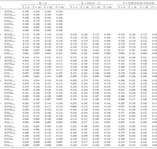
3. The results are reported in Table 5. As for the equal accuracy case, for one-step-ahead

forecasts, we observe that the M DM-based procedures (which are identical for h= 1) and the

DMCI tests display good …nite sample size control. Indeed, theM DM test has almost no size

distortions even for small T, while only a very modest amount of under-size is displayed for

DMCI;1 and DMCI;2. On the other hand, DMBart is over-sized, particularly for the smaller

sample sizes. When h > 1, we …nd a similar picture of size behaviour to that in Table 3.

Speci…cally, M DMrej and DMBart can be substantially over-sized, although the over-size of

M DMrej is less severe than for the equal accuracy case, since here the encompassing test is

conducted against a one-sided alternative, hence only a proportion of the negative long-run

variances obtained induce a rejection of the null. Of the M DM-based approaches, M DMnon

o¤ers the best size control with size always below 0.14, whileM DMSRandM DMBsu¤er from

greater size distortion, although to a lesser extent than was found in the equal accuracy testing

context. DMCI;1 and DMCI;2 again have very good size behaviour across most settings, the

exceptions being when the errors are highly serially correlated and eitherT = 16together with

h = 5 or h = 6, where DMCI;1 and DMCI;2 can su¤er from a small amount of upward size

distortion, or T = 8 and h >2, in which case DMCI;1 can again be over-sized, whileDMCI;2

o¤ers greater size control in these cases.

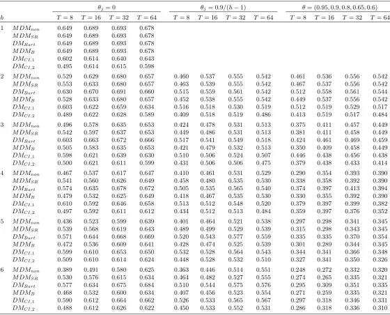
Turning to power for forecast encompassing tests, Table 6 gives results for the size-adjusted

powers ofM DMnon,M DMSR,DMBart,M DMB,DMCI;1 and DMCI;2 for the relevant DGPs

of section 3, withkvarying acrossT as speci…ed in that section; the critical values used for the size-adjustment are again obtained by simulation from the corresponding size experiment. The

relative power rankings of the tests are unchanged compared to tests for equal forecast accuracy,

therefore the comments and conclusions outlined above are equally applicable in this context.

We again …nd thatM DM has a power advantage over theDMCI tests forh= 1, whileDMCI;1

generally outperforms the other procedures for T = 8 and h > 1, and for the longer forecast

horizons when T is larger. DMCI;2 again has generally lower power than DMCI;1, although

this is only of real import when T = 8. Once again, therefore, M DM is to be recommended for one-step-ahead forecasts, but for multi-step-ahead forecasts, apart from a potential role for

M DMnon when a simple M DM-based modi…cation is desired, it is the DMCI;1 and DMCI;2

tests that are to be preferred. These tests o¤er the best …nite sample performance in terms

of size and relative power, with DMCI;2 recommended for T = 8 when h > 2, and DMCI;1

6

Simulations calibrated from empirical data

In order to ensure that our simulation results are representative of what is likely to be

en-countered in practical applications, we now consider a set of simulations for a DGP where the

sample sizes, forecast horizons and forecast error serial correlation settings are all calibrated

according to a particular application in the literature. Speci…cally, we follow the Dreger and

Wolters (2014) application where Euro-area in‡ation is forecast one, two and three years ahead

from an autoregressive model using quarterly data. We obtained HICP in‡ation data from the

authors for the period 1981Q1–2010Q4, and, following Dreger and Wolters, we construct 1-, 4-,

8- and 12-quarter in‡ation rates as follows

h t =

4

hlog(pct=pct h); h= 1;4;8;12

wherepctdenotes the consumer price index (HICP). The forecasting equation uses the

bench-mark model of Dreger and Wolters, based on prediction using current and lagged quarterly

in‡ation:

h

t+h = 1 1t + 2 1t 1+ 3 1t 2+ 4 1t 3+"t+h: (4)

Following Dreger and Wolters, at each forecast horizon we …rst estimate the model over the

initial in-sample period 1983Q1–2002Q4. The parameter estimates are then used to produce

the …rst h = 4, h = 8 and h = 12 forecasts for the periods 2003Q4, 2004Q4 and 2005Q4, respectively. The in-sample period is then extended by one observation and (4) is re-estimated,

with the results used to obtain the next forecast for 2004Q1 at h = 4, 2005Q1 at h = 8 and

2006Q1 at h = 12. Continuing in this recursive manner, the …nal forecast for each forecast horizon is obtained for time 2010Q4, therefore producing a total of T = 29forecasts forh= 4,

T = 25 forh = 8, and T = 21 for h= 12. Denoting the forecast at a given time and horizon by ^h_t+h, we can obtain three forecast error series

eh_t+h= h_t+h ^h_t+h; h= 4;8;12:

To determine the degree of serial correlation present in the forecast errors, we …t moving average

processes to the three forecast error series, determining the order of MA process in each case

according to the Akaike information criterion, selecting from MA processes up to order h 1. We …nd the selected models to be M A(3), M A(2) and M A(4) for h = 4, h = 8 and h = 12,

respectively, with the …tted MA coe¢ cients given in Table 7. Although these MA parameters

have been estimated using a very small sample size, it can be seen that the values obtained are

not inconsistent with the settings adopted in the earlier simulation exercises.

Given the calibrations obtained from the Dreger and Wolters application, we repeat the

sim-ulation experiments considered in sections 3 and 5, but now with the settingsT =_f29;25;21_g,

h = _f4;8;12_g and the corresponding j values from Table 7. Accordingly, Table 8 reports

the frequency with which negative long-run variance estimates arise when using the standard

under both the respective null and alternative hypotheses. The settings under the alternative

for the three horizon/sample size pairings considered are R=_f4;6;8_g (for testing equal

accu-racy) and k=_f2;1:8;1:8_g (for encompassing testing), again chosen so that the test powers are broadly comparable across sample sizes. For h= 4, we observe a very low occurrence of

neg-ative long-run variance estimates, while for h = 8 the proportion of negative estimates across the simulations is in the region of 0.15, rising to around 0.33 for h = 12. These comments apply equally to tests for equal forecast accuracy and tests for forecast encompassing. The

sample sizes considered in this empirically calibrated exercise lie inbetween the T = 16 and

T = 32 settings used in the section 3 simulations, and two of the forecast horizons considered

are greater than the range considered in section 3. However, it is clear that the pattern of

frequencies for negative estimates is consistent with the earlier results, with a high incidence

of problematic negative outcomes as the forecast horizon increases. This further demonstrates

that the possibility of obtaining a negative long-run variance estimate is an empirically relevant

issue when applying standard tests for equal accuracy and encompassing in small samples.

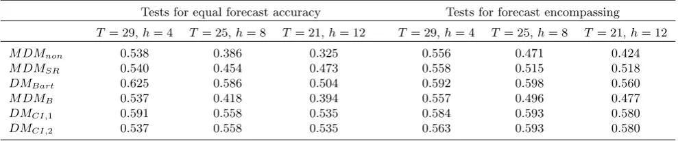
Table 9 presents the empirical sizes of the di¤erent test procedures for the empirically

calibrated settings. Note that DMCI;1 and DMCI;2 are identical when T = 25 (h = 8) and

T = 21 (h = 12), hence di¤erences are only seen for the h = 4 results where T = 29. The

DMCI tests clearly o¤er the best size control of the procedures considered for tests for equal

forecast accuracy and forecast encompassing, and the two bandwidth settings in DMCI;1 and

DMCI;2 deliver similar size results. Given that here we consider longer forecast horizons than

in section 5, it is reassuring to see thatDMCI;1 andDMCI;2 retain good size control acrossh.

As would be expected given the earlier simulations, substantial over-size is seen for M DMrej

and DMBart, particularly for the longer forecast horizons. Of the other M DM-based tests,

M DMnon o¤ers the best size control as before, with a maximum size around 0.15 observed,

while M DMSR and M DMB can have size up to around 0.19 and 0.24 respectively. Table 10

reports the corresponding size-adjusted powers of the procedures, and, with the exception of

the badly over-sized DMBart test, DMCI;1 displays the best power performance, followed by

DMCI;2. In contrast, the best-sizedM DM-based procedure,M DMnon, su¤ers from relatively

low size-adjusted power forh= 8 andh= 12. These results clearly strengthen the case for use of DMCI;1 orDMCI;2 in practical applications.

7

Impact of model parameter estimation uncertainty

Beginning primarily with West (1996), much work on forecast evaluation testing has focused on

cases where the forecasts have been produced by estimated models, either non-nested or nested,

and more sophisticated methods have been proposed to properly account for the impact that

model parameter estimation uncertainty can have on the distributions of DM-type forecast

accuracy and encompassing tests in such circumstances. For reviews of this literature, see West

from estimated models, the original DM approach is asymptotically valid without the need for

any modi…cation. Examples are where the forecast models are non-nested, linear and estimated

by ordinary least squares (OLS), along with the loss function being mean squared forecast error,

or when the number of forecast observations is small relative to the number of observations used

for model estimation. In this section, we consider a set of simulations designed to examine the

same issues of negative long-run variance estimation and test size performance in small samples,

but now where the forecasts have …rst been obtained from estimated models. In order to focus

on tests that are asymptotically valid, we restrict attention to tests for equal mean squared

forecast error where the forecasts are obtained from non-nested linear models estimated by

OLS.

Our forecasting exercise involves an in-sample period for model estimation,t= 1; :::; N, and

an out-of-sample period for forecast evaluation,t=N+ 1; :::; N+T. We consider the following DGP

yt= 1x1t+ 2x2t+"t; t= 1; :::; N +T

where, without loss of generality, we interpret x1t and x2t to be predictor variables useful for

forecasting yt at horizon h. We set [x1t; x2t]0 N(0; I2) and, as our focus here is on the

impact of parameter estimation uncertainty rather than forecast error serial correlation, we

simply generate "t N(0;1), t = 1; :::; N +T, independently of [x1t; x2t]0. As in the j = 0

simulations of sections 3 and 5, we do not assume knowledge of this lack of serial correlation

when constructing the test statistics, so the results can be compared directly with the j = 0

sections of Tables 1 and 3. We consider two model-based forecasts, with the models given by

Model 1 : yt= 1x1t+e1t

Model 2 : yt= 2x2t+e2t

which are …rst estimated by OLS over the period t= 1; :::; N to give the parameter estimates ^

1 and ^2. The two forecast series are then speci…ed as

f1t = ^1x1t; t=N + 1; :::; N+T

f2t = ^2x2t; t=N + 1; :::; N+T

with the corresponding forecast errors

^

e1t = yt ^1x1t

^

e2t = yt ^2x2t:

The tests for equal forecast accuracy are then de…ned exactly as in section 4, but withe1t and

e2treplaced withe^1tande^2t, respectively. By setting 1 = 2, it is straightforward to show that

sizes, N = 40 and N = 80, combined with the same set of out-of-sample sizes and forecast horizons employed in the earlier simulations of sections 3 and 5.

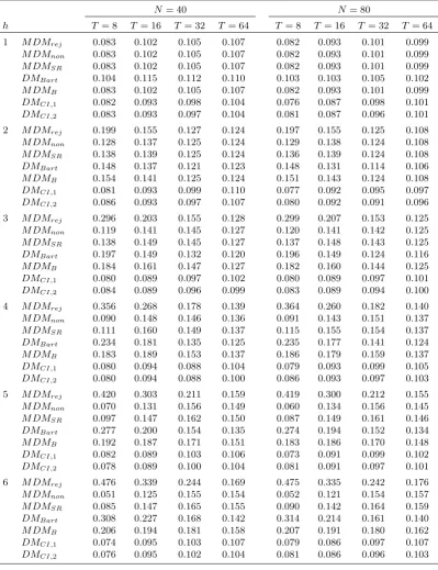
Table 11 reports results for the frequency of negative long-run variance estimates. On

comparing these results (for both N = 40 and N = 80) with the j = 0 section of Panel A

of Table 1, we …nd that the results are almost identical, hence the presence of forecast model

parameter estimation uncertainty has almost no e¤ect on the prevalence of negative estimates.

Table 12 gives results for the empirical sizes of the test procedures, and while some minor

di¤erences are seen between the results forN = 40andN = 80, the results for the di¤erent in-sample sizes are broadly similar to each other, and there is little di¤erence between these results

and those for j = 0in Table 3. Once again, therefore, the impact of estimating the forecast

models is very slight, and the same comments made in section 5 apply here. The fundamental

…ndings of (i) a high frequency of negative long-run variance estimates when evaluating

multi-step-ahead forecasts using small numbers of out-of-sample forecast errors, and (ii) the DMCI

tests o¤ering the best size control among the alternative procedures considered, are therefore

equally relevant in the context of forecasts obtained from estimated models.

8

Conclusion

In this paper, we have highlighted that application of the standard DM-based tests for equal

forecast accuracy and forecast encompassing can often result in a negative long-run variance

estimate when dealing with multi-step-ahead predictions and small, but empirically relevant,

sample sizes. Having examined a number of possible approaches to dealing with this

prob-lem, we have found that the recently proposed testing approach of Coroneo and Iacone (2016),

which uses a weighted periodogram long-run variance estimator combined with …xed-bandwidth

asymptotics, o¤ers the best overall …nite sample size and power performance. Use of this test

with a bandwidth setting of T1=3 or T1=4 (the choice being determined by the sample size and forecast horizon involved) results in only modest size distortions, while power levels are

appealing relative to other approaches, permitting reliable inference even in the small

sam-ple/long horizon cases we consider. Aside from this preferred approach, a case could possibly

be made for a strategy that uses theM DM tests of Harveyet al. (1997, 1998) when a positive long-run variance estimate is obtained, and defaulting to a non-rejection of the null hypothesis

when a negative long-run variance arises; while this approach does not perform as well as the

Coroneo and Iacone (2016) procedure, it does have the advantage of simplicity, since no

ad-ditional computation beyond calculation of the M DM statistic is required. Finally, when the

forecast evaluation is being done with one-step-ahead predictions, no negative long-run variance

estimates can arise with the standard tests, and the M DM tests provide good size control and

superior power to the Coroneo and Iacone (2016) test.

The simulations conducted in this paper considered a range of sample sizes and forecast

focused throughout on normally distributed forecast errors, we also considered simulations based

on errors drawn from thet6 distribution, given that forecast errors often appear to display

fat-tailed behaviour. We found the results to be qualitatively similar to those based on normal

errors, hence our conclusions would be unchanged under such a forecast error assumption.

Finally, we note that the issue of negative long-run variance estimates would also be relevant

in the recommended test of Harvey and Newbold (2000) for multiple forecast encompassing

(where the null is that one forecast encompasses a number of competing predictors), since

this test employs a multivariate version of the M DM approach. It would be expected that the variance-covariance estimator in the test statistic could fail to be positive de…nite for small

samples and multi-step-ahead predictions, and in future work it would be interesting to consider

extensions of the above techniques to that context.

References

Andrews, D.W.K. (1991). Heteroskedasticity and autocorrelation consistent covariance matrix

estimation. Econometrica, 59, 817–858.

Andrews, D.W.K. and Monahan, J.C. (1992). An improved heteroskedasticity and

autocorre-lation consistent covariance matrix estimator. Econometrica, 60, 953–966.

Ashley, R. (2003). Statistically signi…cant forecasting improvements: how much out-of-sample

data is likely necessary? International Journal of Forecasting, 19, 229–239.

Ashley, R. and Tsang, K.P. (2014). Credible Granger-causality inference with modest sample

lengths: a cross-sample validation approach. Econometrics, 2, 72–91.

Bates, J.M. and Granger, C.W.J. (1969). The combination of forecasts. Operational Research

Quarterly, 20, 451–468.

Caporale, G.M. and Gil-Alana, L. (2014). Long-run and cyclical dynamics in the US stock

market. Journal of Forecasting, 33, 147–161.

Chow, H.K. and Choy, K.M. (2006). Forecasting the global electronics cycle with leading

indicators: A Bayesian VAR approach. International Journal of Forecasting, 22, 301–

315.

Clark, T.E. (1999). Finite-sample properties of tests for equal forecast accuracy. Journal of

Forecasting, 18, 489–504.

Clark, T.E. and McCracken, M. (2013). Advances in forecast evaluation. In Handbook of

Economic Forecasting, Vol. 2, Part B, Elliott, G. and Timmerman, A. (eds.), pp. 1107–

Clements, M.P. and Harvey, D.I. (2009). Forecast combination and encompassing. InPalgrave

Handbook of Econometrics, Vol. 2: Applied Econometrics, Mills, T.C. and Patterson, K.

(eds.), pp. 169–198, Palgrave Macmillan, Basingstoke.

Coroneo, L. and Iacone, F. (2016). Comparing predictive accuracy in small samples using

…xed-smoothing asymptotics. Discussion Paper, Department of Economics, University of

York.

Dib, A., Gammoudi, M. and Moran, K. (2008). Forecasting Canadian time series with the

New Keynesian model. Canadian Journal of Economics, 41, 138–165.

Diebold, F.X. and Mariano, R.S. (1995). Comparing predictive accuracy. Journal of Business

and Economics Statistics, 13, 253–263.

Dreger, C. and Wolters, J. (2014). Money demand and the role of monetary indicators in

forecasting euro area in‡ation. International Journal of Forecasting, 30, 303–312.

Harvey, D.I., Leybourne, S.J. and Newbold, P. (1997). Testing the equality of prediction mean

squared errors. International Journal of Forecasting, 13 281–291.

Harvey, D.I., Leybourne, S.J. and Newbold, P. (1998). Tests for forecast encompassing.

Jour-nal of Business and Economic Statistics, 16, 254–259.

Harvey, D.I., Leybourne, S.J. and Newbold, P. (1999). Forecast evaluation tests in the presence

of ARCH.Journal of Forecasting, 18, 435–445.

Harvey, D.I. and Newbold, P. (2000). Tests for multiple forecast encompassing. Journal of

Applied Econometrics, 15, 471–482.

Hering, A.S. and Genton, M.G. (2011). Comparing spatial predictions. Technometrics, 53,

414–425.

Hualde, J. and Iacone, F. (2017). Fixed bandwidth asymptotics for the studentized mean of

fractionally integrated processes. Economics Letters, 150, 39–43.

Mehl, A. (2009). The yield curve as a predictor and emerging economies. Open Economies

Review, 20, 683–716.

Qin, D., Cagas, M.A., Ducanes, G., Magtibay-Ramos, N. and Quising, P. (2008). Automatic

leading indicators versus macroeconometric structural models: A comparison of in‡ation

and GDP growth forecasting. International Journal of Forecasting, 24, 399–413.

West, K.D. (1996). Asymptotic inference about predictive ability. Econometrica, 64, 1067–

1084.

West, K.D. (2006). Forecast evaluation. InHandbook of Economic Forecasting, Vol. 1, Elliott,

Table 1. Frequency of negative long-run variance estimates in tests for equal forecast accuracy.

θj= 0 θj= 0.9/(h−1) θ= (0.95,0.9,0.8,0.65,0.6)

h T = 8 T = 16 T = 32 T = 64 T = 8 T = 16 T= 32 T = 64 T = 8 T = 16 T = 32 T = 64

Panel A.R= 1 (null)

2 0.074 0.015 0.001 0.000 0.036 0.003 0.000 0.000 0.035 0.004 0.000 0.000

3 0.175 0.064 0.013 0.000 0.131 0.032 0.003 0.000 0.101 0.019 0.002 0.000

4 0.275 0.120 0.031 0.002 0.231 0.077 0.016 0.001 0.182 0.047 0.004 0.000

5 0.352 0.175 0.055 0.008 0.325 0.141 0.034 0.004 0.297 0.081 0.012 0.001

6 0.422 0.217 0.085 0.017 0.406 0.186 0.060 0.008 0.367 0.121 0.024 0.001

Panel B.R >1(alternative)

2 0.057 0.007 0.001 0.000 0.038 0.002 0.000 0.000 0.037 0.002 0.000 0.000

3 0.169 0.052 0.009 0.000 0.134 0.028 0.003 0.000 0.113 0.016 0.001 0.000

4 0.268 0.107 0.027 0.002 0.228 0.075 0.015 0.000 0.191 0.047 0.004 0.000

5 0.347 0.166 0.052 0.007 0.331 0.135 0.033 0.004 0.310 0.081 0.011 0.001

6 0.430 0.211 0.085 0.016 0.414 0.189 0.060 0.007 0.368 0.130 0.024 0.001

Table 2. Frequency of negative long-run variance estimates in tests for forecast encompassing.

θj= 0 θj= 0.9/(h−1) θ= (0.95,0.9,0.8,0.65,0.6)

h T = 8 T = 16 T = 32 T = 64 T = 8 T = 16 T= 32 T = 64 T = 8 T = 16 T = 32 T = 64

Panel A.ρ= 1(null)

2 0.070 0.015 0.001 0.000 0.037 0.003 0.000 0.000 0.036 0.003 0.000 0.000

3 0.182 0.067 0.012 0.001 0.130 0.030 0.002 0.000 0.104 0.018 0.001 0.000

4 0.275 0.126 0.029 0.003 0.226 0.083 0.014 0.001 0.177 0.045 0.005 0.000

5 0.360 0.169 0.054 0.009 0.330 0.132 0.033 0.002 0.306 0.081 0.010 0.000

6 0.424 0.220 0.089 0.017 0.406 0.180 0.061 0.008 0.360 0.126 0.021 0.002

Panel B.ρ <1(alternative)

2 0.063 0.012 0.001 0.000 0.033 0.003 0.000 0.000 0.034 0.003 0.000 0.000

3 0.169 0.054 0.009 0.000 0.129 0.029 0.002 0.000 0.105 0.020 0.001 0.000

4 0.263 0.116 0.027 0.003 0.221 0.081 0.012 0.001 0.190 0.044 0.003 0.000

5 0.349 0.166 0.051 0.008 0.331 0.132 0.032 0.002 0.300 0.084 0.011 0.000

Table 3. Empirical size of nominal 0.10-level tests for equal forecast accuracy.

θj= 0 θj= 0.9/(h−1) θ= (0.95,0.9,0.8,0.65,0.6)

h T= 8 T = 16 T = 32 T = 64 T = 8 T= 16 T = 32 T = 64 T = 8 T = 16 T= 32 T = 64

1 M DMrej 0.085 0.091 0.102 0.103

M DMnon 0.085 0.091 0.102 0.103

M DMSR 0.085 0.091 0.102 0.103

DMBart 0.107 0.103 0.108 0.105

M DMB 0.085 0.091 0.102 0.103

DMCI,1 0.085 0.087 0.099 0.098

DMCI,2 0.086 0.087 0.097 0.097

2 M DMrej 0.203 0.145 0.124 0.109 0.165 0.123 0.116 0.107 0.164 0.122 0.116 0.107

M DMnon 0.129 0.130 0.123 0.109 0.129 0.120 0.116 0.107 0.129 0.119 0.116 0.107

M DMSR 0.137 0.131 0.123 0.109 0.135 0.120 0.116 0.107 0.136 0.119 0.116 0.107

DMBart 0.150 0.125 0.118 0.107 0.185 0.158 0.154 0.142 0.186 0.159 0.155 0.142

M DMB 0.153 0.133 0.123 0.109 0.144 0.121 0.116 0.107 0.144 0.120 0.116 0.107

DMCI,1 0.081 0.086 0.095 0.102 0.092 0.086 0.097 0.099 0.092 0.085 0.097 0.099

DMCI,2 0.086 0.086 0.097 0.101 0.079 0.086 0.096 0.095 0.079 0.085 0.096 0.094

3 M DMrej 0.294 0.207 0.153 0.122 0.256 0.183 0.134 0.113 0.235 0.167 0.126 0.112

M DMnon 0.119 0.143 0.140 0.122 0.125 0.150 0.131 0.112 0.134 0.148 0.124 0.112

M DMSR 0.138 0.150 0.142 0.122 0.145 0.156 0.132 0.112 0.159 0.153 0.124 0.112

DMBart 0.193 0.151 0.130 0.114 0.234 0.193 0.162 0.146 0.261 0.209 0.175 0.159

M DMB 0.183 0.163 0.144 0.122 0.180 0.163 0.132 0.112 0.187 0.157 0.124 0.112

DMCI,1 0.082 0.092 0.094 0.098 0.109 0.099 0.100 0.097 0.120 0.094 0.094 0.095

DMCI,2 0.083 0.092 0.094 0.095 0.087 0.099 0.089 0.092 0.086 0.094 0.087 0.089

4 M DMrej 0.366 0.263 0.179 0.131 0.340 0.229 0.158 0.117 0.321 0.207 0.139 0.115

M DMnon 0.090 0.143 0.148 0.128 0.108 0.144 0.142 0.116 0.139 0.160 0.135 0.115

M DMSR 0.112 0.157 0.151 0.128 0.136 0.156 0.144 0.116 0.192 0.174 0.136 0.115

DMBart 0.230 0.178 0.139 0.114 0.272 0.204 0.169 0.145 0.341 0.248 0.194 0.166

M DMB 0.183 0.183 0.157 0.129 0.196 0.173 0.147 0.117 0.233 0.182 0.137 0.115

DMCI,1 0.074 0.091 0.095 0.092 0.108 0.100 0.097 0.093 0.153 0.101 0.097 0.098

DMCI,2 0.079 0.091 0.097 0.094 0.085 0.100 0.088 0.089 0.079 0.101 0.086 0.088

5 M DMrej 0.415 0.304 0.215 0.150 0.404 0.282 0.187 0.136 0.406 0.246 0.165 0.134

M DMnon 0.063 0.130 0.160 0.142 0.079 0.141 0.153 0.132 0.110 0.164 0.153 0.133

M DMSR 0.091 0.147 0.165 0.143 0.118 0.162 0.157 0.132 0.218 0.198 0.157 0.133

DMBart 0.269 0.191 0.150 0.123 0.313 0.229 0.176 0.153 0.410 0.278 0.217 0.186

M DMB 0.186 0.182 0.173 0.144 0.207 0.192 0.161 0.133 0.280 0.206 0.158 0.133

DMCI,1 0.079 0.093 0.097 0.097 0.107 0.106 0.103 0.099 0.198 0.108 0.103 0.102

DMCI,2 0.080 0.093 0.096 0.100 0.096 0.106 0.096 0.094 0.083 0.108 0.088 0.093

6 M DMrej 0.469 0.340 0.239 0.165 0.463 0.320 0.216 0.148 0.452 0.277 0.187 0.136

M DMnon 0.047 0.123 0.154 0.148 0.056 0.134 0.156 0.140 0.085 0.156 0.163 0.135

M DMSR 0.082 0.145 0.161 0.150 0.101 0.159 0.165 0.141 0.240 0.208 0.172 0.135

DMBart 0.301 0.227 0.162 0.129 0.350 0.250 0.184 0.151 0.474 0.312 0.236 0.188

M DMB 0.193 0.196 0.176 0.153 0.221 0.202 0.174 0.142 0.311 0.218 0.173 0.135

DMCI,1 0.077 0.092 0.100 0.097 0.102 0.106 0.111 0.100 0.241 0.118 0.107 0.100

Table 4. Size-adjusted power of nominal 0.10-level tests for equal forecast accuracy.

θj= 0 θj= 0.9/(h−1) θ= (0.95,0.9,0.8,0.65,0.6)

h T= 8 T = 16 T = 32 T = 64 T = 8 T= 16 T = 32 T = 64 T = 8 T = 16 T= 32 T = 64

1 M DMnon 0.710 0.820 0.677 0.699

M DMSR 0.710 0.820 0.677 0.699

DMBart 0.710 0.820 0.677 0.699

M DMB 0.710 0.820 0.677 0.699

DMCI,1 0.564 0.655 0.591 0.642

DMCI,2 0.357 0.655 0.528 0.555

2 M DMnon 0.454 0.688 0.638 0.679 0.396 0.594 0.521 0.559 0.384 0.595 0.520 0.556

M DMSR 0.480 0.689 0.638 0.679 0.404 0.596 0.521 0.559 0.402 0.596 0.520 0.556

DMBart 0.646 0.795 0.673 0.689 0.535 0.669 0.542 0.560 0.531 0.655 0.540 0.559

M DMB 0.443 0.686 0.638 0.679 0.389 0.596 0.521 0.559 0.384 0.593 0.520 0.556

DMCI,1 0.609 0.648 0.606 0.612 0.511 0.545 0.471 0.499 0.497 0.545 0.472 0.500

DMCI,2 0.374 0.648 0.533 0.538 0.326 0.545 0.416 0.438 0.330 0.545 0.416 0.437

3 M DMnon 0.385 0.574 0.601 0.656 0.340 0.479 0.466 0.509 0.283 0.399 0.390 0.420

M DMSR 0.433 0.596 0.605 0.656 0.376 0.490 0.466 0.509 0.305 0.401 0.390 0.420

DMBart 0.565 0.757 0.679 0.689 0.466 0.596 0.515 0.525 0.363 0.483 0.419 0.431

M DMB 0.393 0.565 0.601 0.656 0.349 0.478 0.465 0.509 0.287 0.396 0.389 0.420

DMCI,1 0.564 0.635 0.619 0.643 0.468 0.526 0.460 0.487 0.394 0.431 0.387 0.400

DMCI,2 0.374 0.635 0.556 0.558 0.307 0.526 0.437 0.415 0.290 0.431 0.346 0.352

4 M DMnon 0.388 0.505 0.531 0.638 0.339 0.441 0.454 0.523 0.249 0.310 0.303 0.361

M DMSR 0.506 0.561 0.540 0.639 0.401 0.466 0.459 0.523 0.278 0.315 0.301 0.361

DMBart 0.570 0.717 0.652 0.682 0.467 0.580 0.528 0.551 0.310 0.392 0.339 0.380

M DMB 0.428 0.524 0.535 0.638 0.353 0.429 0.456 0.523 0.249 0.308 0.301 0.361

DMCI,1 0.604 0.627 0.592 0.647 0.493 0.525 0.486 0.512 0.340 0.373 0.324 0.347

DMCI,2 0.389 0.627 0.529 0.571 0.332 0.525 0.451 0.460 0.256 0.373 0.300 0.310

5 M DMnon 0.389 0.476 0.483 0.599 0.319 0.413 0.436 0.516 0.197 0.235 0.259 0.294

M DMSR 0.513 0.556 0.507 0.603 0.425 0.462 0.448 0.518 0.232 0.241 0.257 0.294

DMBart 0.560 0.698 0.647 0.679 0.467 0.580 0.531 0.554 0.266 0.308 0.298 0.314

M DMB 0.418 0.517 0.498 0.602 0.364 0.428 0.446 0.519 0.243 0.235 0.256 0.294

DMCI,1 0.592 0.629 0.598 0.626 0.503 0.516 0.507 0.524 0.281 0.314 0.288 0.305

DMCI,2 0.395 0.629 0.533 0.526 0.322 0.516 0.444 0.448 0.234 0.314 0.261 0.257

6 M DMnon 0.318 0.441 0.461 0.577 0.297 0.387 0.397 0.505 0.185 0.225 0.205 0.267

M DMSR 0.505 0.545 0.488 0.581 0.419 0.471 0.417 0.506 0.193 0.230 0.203 0.268

DMBart 0.546 0.677 0.618 0.681 0.482 0.589 0.519 0.561 0.219 0.268 0.250 0.280

M DMB 0.433 0.506 0.482 0.583 0.374 0.429 0.405 0.505 0.202 0.227 0.201 0.267

DMCI,1 0.597 0.632 0.583 0.638 0.495 0.552 0.491 0.533 0.224 0.288 0.247 0.279

Table 5. Empirical size of nominal 0.10-level tests for forecast encompassing.

θj= 0 θj= 0.9/(h−1) θ= (0.95,0.9,0.8,0.65,0.6)

h T= 8 T = 16 T = 32 T = 64 T = 8 T= 16 T = 32 T = 64 T = 8 T = 16 T= 32 T = 64

1 M DMrej 0.100 0.100 0.102 0.103

M DMnon 0.100 0.100 0.102 0.103

M DMSR 0.100 0.100 0.102 0.103

DMBart 0.142 0.119 0.111 0.108

M DMB 0.100 0.100 0.102 0.103

DMCI,1 0.091 0.095 0.102 0.103

DMCI,2 0.088 0.095 0.098 0.100

2 M DMrej 0.153 0.130 0.110 0.110 0.138 0.120 0.112 0.108 0.138 0.120 0.112 0.108

M DMnon 0.118 0.123 0.110 0.110 0.119 0.118 0.112 0.108 0.119 0.118 0.112 0.108

M DMSR 0.125 0.125 0.110 0.110 0.124 0.119 0.112 0.108 0.125 0.119 0.112 0.108

DMBart 0.174 0.136 0.116 0.112 0.170 0.151 0.136 0.131 0.170 0.151 0.137 0.131

M DMB 0.134 0.126 0.110 0.110 0.129 0.119 0.112 0.108 0.129 0.119 0.112 0.108

DMCI,1 0.095 0.097 0.098 0.102 0.110 0.101 0.105 0.107 0.111 0.101 0.106 0.107

DMCI,2 0.094 0.097 0.095 0.101 0.094 0.101 0.094 0.099 0.093 0.101 0.094 0.099

3 M DMrej 0.184 0.151 0.131 0.111 0.171 0.145 0.121 0.115 0.163 0.140 0.121 0.114

M DMnon 0.094 0.119 0.125 0.111 0.106 0.129 0.120 0.115 0.110 0.131 0.120 0.114

M DMSR 0.113 0.127 0.126 0.111 0.124 0.133 0.121 0.115 0.131 0.133 0.120 0.114

DMBart 0.189 0.147 0.130 0.114 0.192 0.166 0.147 0.135 0.206 0.178 0.157 0.142

M DMB 0.135 0.133 0.127 0.111 0.139 0.136 0.121 0.115 0.141 0.135 0.120 0.114

DMCI,1 0.095 0.095 0.104 0.105 0.121 0.105 0.106 0.106 0.130 0.106 0.108 0.106

DMCI,2 0.088 0.095 0.101 0.099 0.090 0.105 0.099 0.098 0.089 0.106 0.100 0.097

4 M DMrej 0.214 0.181 0.134 0.116 0.202 0.174 0.131 0.118 0.206 0.161 0.128 0.121

M DMnon 0.076 0.116 0.121 0.115 0.095 0.132 0.123 0.118 0.118 0.137 0.125 0.121

M DMSR 0.105 0.132 0.123 0.116 0.123 0.144 0.125 0.118 0.154 0.147 0.127 0.121

DMBart 0.207 0.169 0.128 0.116 0.212 0.180 0.146 0.140 0.251 0.208 0.166 0.154

M DMB 0.141 0.146 0.126 0.116 0.150 0.152 0.126 0.118 0.172 0.150 0.127 0.121

DMCI,1 0.093 0.106 0.100 0.098 0.123 0.116 0.107 0.108 0.166 0.117 0.111 0.113

DMCI,2 0.091 0.106 0.097 0.097 0.101 0.116 0.100 0.102 0.090 0.117 0.100 0.104

5 M DMrej 0.235 0.187 0.144 0.120 0.225 0.182 0.140 0.116 0.227 0.178 0.138 0.119

M DMnon 0.057 0.102 0.117 0.115 0.060 0.115 0.124 0.116 0.075 0.136 0.133 0.119

M DMSR 0.092 0.122 0.123 0.115 0.103 0.134 0.129 0.116 0.154 0.158 0.135 0.119

DMBart 0.222 0.173 0.136 0.114 0.222 0.184 0.148 0.130 0.271 0.226 0.174 0.152

M DMB 0.142 0.141 0.130 0.116 0.146 0.148 0.133 0.116 0.178 0.163 0.135 0.119

DMCI,1 0.092 0.098 0.100 0.098 0.113 0.117 0.108 0.103 0.182 0.131 0.117 0.108

DMCI,2 0.086 0.098 0.098 0.092 0.099 0.117 0.101 0.095 0.097 0.131 0.100 0.099

6 M DMrej 0.251 0.207 0.163 0.125 0.255 0.198 0.158 0.122 0.253 0.195 0.141 0.124

M DMnon 0.044 0.095 0.116 0.117 0.051 0.107 0.126 0.117 0.070 0.128 0.131 0.123

M DMSR 0.086 0.118 0.125 0.119 0.103 0.135 0.135 0.118 0.170 0.165 0.135 0.123

DMBart 0.248 0.183 0.141 0.115 0.248 0.196 0.160 0.132 0.307 0.243 0.182 0.159

M DMB 0.148 0.143 0.134 0.120 0.164 0.153 0.140 0.119 0.198 0.171 0.136 0.123

DMCI,1 0.095 0.099 0.099 0.095 0.116 0.117 0.116 0.103 0.214 0.144 0.125 0.111

Table 6. Size-adjusted power of nominal 0.10-level tests for forecast encompassing.

θj= 0 θj= 0.9/(h−1) θ= (0.95,0.9,0.8,0.65,0.6)

h T= 8 T = 16 T = 32 T = 64 T = 8 T= 16 T = 32 T = 64 T = 8 T = 16 T= 32 T = 64

1 M DMnon 0.649 0.689 0.693 0.678

M DMSR 0.649 0.689 0.693 0.678

DMBart 0.649 0.689 0.693 0.678

M DMB 0.649 0.689 0.693 0.678

DMCI,1 0.602 0.614 0.640 0.643

DMCI,2 0.495 0.614 0.615 0.598

2 M DMnon 0.529 0.629 0.680 0.657 0.460 0.537 0.555 0.542 0.461 0.536 0.556 0.542

M DMSR 0.553 0.633 0.680 0.657 0.463 0.539 0.555 0.542 0.467 0.537 0.556 0.542

DMBart 0.630 0.670 0.691 0.660 0.515 0.559 0.561 0.542 0.512 0.558 0.561 0.544

M DMB 0.528 0.633 0.680 0.657 0.452 0.538 0.555 0.542 0.449 0.537 0.556 0.542

DMCI,1 0.603 0.622 0.659 0.634 0.516 0.518 0.530 0.519 0.512 0.519 0.529 0.517

DMCI,2 0.489 0.622 0.628 0.589 0.409 0.518 0.519 0.486 0.413 0.519 0.517 0.484

3 M DMnon 0.496 0.578 0.635 0.653 0.424 0.478 0.531 0.513 0.375 0.411 0.457 0.449

M DMSR 0.542 0.597 0.637 0.653 0.449 0.486 0.531 0.513 0.381 0.411 0.458 0.449

DMBart 0.603 0.663 0.672 0.666 0.517 0.541 0.549 0.518 0.424 0.461 0.469 0.459

M DMB 0.505 0.583 0.635 0.653 0.421 0.479 0.532 0.513 0.350 0.409 0.458 0.449

DMCI,1 0.598 0.621 0.639 0.630 0.510 0.506 0.524 0.507 0.446 0.438 0.456 0.438

DMCI,2 0.500 0.621 0.611 0.599 0.431 0.506 0.506 0.475 0.379 0.438 0.433 0.414

4 M DMnon 0.467 0.537 0.617 0.647 0.410 0.461 0.531 0.529 0.290 0.354 0.393 0.390

M DMSR 0.541 0.560 0.626 0.649 0.458 0.480 0.535 0.530 0.338 0.358 0.392 0.390

DMBart 0.574 0.635 0.678 0.672 0.505 0.535 0.565 0.540 0.374 0.397 0.413 0.394

M DMB 0.479 0.532 0.625 0.649 0.418 0.467 0.535 0.530 0.330 0.355 0.392 0.390

DMCI,1 0.610 0.592 0.646 0.658 0.513 0.512 0.548 0.520 0.379 0.397 0.399 0.382

DMCI,2 0.497 0.592 0.611 0.612 0.434 0.512 0.513 0.484 0.359 0.397 0.376 0.352

5 M DMnon 0.436 0.523 0.599 0.639 0.401 0.464 0.521 0.538 0.297 0.298 0.341 0.345

M DMSR 0.539 0.568 0.619 0.643 0.489 0.499 0.529 0.539 0.315 0.298 0.343 0.345

DMBart 0.571 0.644 0.668 0.669 0.520 0.543 0.577 0.559 0.335 0.335 0.370 0.354

M DMB 0.472 0.536 0.609 0.641 0.428 0.474 0.525 0.539 0.301 0.289 0.344 0.345

DMCI,1 0.599 0.610 0.653 0.650 0.532 0.528 0.564 0.543 0.344 0.341 0.366 0.348

DMCI,2 0.509 0.610 0.614 0.624 0.448 0.528 0.532 0.510 0.327 0.341 0.350 0.326

6 M DMnon 0.389 0.491 0.580 0.625 0.363 0.446 0.514 0.551 0.248 0.272 0.332 0.320

M DMSR 0.530 0.576 0.615 0.634 0.464 0.482 0.527 0.555 0.274 0.265 0.335 0.321

DMBart 0.577 0.634 0.675 0.684 0.510 0.544 0.575 0.576 0.295 0.309 0.351 0.335

M DMB 0.468 0.532 0.600 0.634 0.407 0.456 0.523 0.554 0.271 0.259 0.335 0.321

DMCI,1 0.590 0.612 0.664 0.662 0.526 0.533 0.565 0.567 0.297 0.318 0.346 0.331