1
Comparison of chaos optimization functions for
performance improvement of fitting of
non-linear geometries
Giovanni Moroni
1,2,Wahyudin P. Syam
3,*, and Stefano Petrò
21 School of Mechanical Engineering, Tongji University, 48000 Cao An Road, 201804 Shanghai, P. R.
China
2 Mechanical Engineering Department, Politecnico di Milano, Via La Masa 1, 20156 Milan, Italy 3 Manufacturing Metrology Team, Faculty of Engineering, The University of Nottingham, NG7 2RD,
Nottingham, UK.
*corresponding author: Wahyudin P. Syam ([email protected])
Abstract
Fitting algorithms play an important role in the whole measuring cycle in order to derive a measurement result. They involve associating substitute geometry to a point cloud obtained by an instrument. This situation is more difficult in the case of non-linear geometry fitting since iterative method should be used. This article addresses this problem. Three geometries are selected as relevant case studies: circle, sphere and cylinder. This selection is based on their frequent use in real applications; for example, cylinder is a relevant geometry of an assembly feature such as pin-hole relationship, and spherical geometry is often found as reference geometry in high precision artifacts and mechanisms.
In this article, the use of Chaos optimization (CO) to improve the initial solution to feed the iterative Levenberg-Marquardt (LM) algorithm to fit non-linear geometries is considered. A previous paper has shown the performance of this combination in improving the fitting of both complete and incomplete geometries. This article focuses on the comparison of the efficiency of different one-dimensional maps of CO. This study shows that, in general, logistic-map function provides the best solution compared to other types of one-dimensional functions. Finally, case studies on hemispheres and industrial cylinders fitting are presented.
Keywords: Least-square fitting, non-linear optimization, chaos optimization, one dimensional map.
1. Introduction
2
roundness, parallelism, coaxiality deviations, are performed accurately and flexibly. Therefore, the fitting algorithm is a fundamental element in the whole chain of dimensional metrology. Based on Hoppe et. al. [6], fitting the substitute geometry is called a “function reconstruction”, since it is an association of points to a defined function. From the point of view of the fitting algorithm, basic geometries can be divided in two groups: linear and non-linear. Linear geometries include 2D line and plane. Most other types of basic geometries, such as circle, sphere, cylinder, and cone are considered non-linear geometries.
The fitting of linear geometries can be analytically solved and a single global optimal result obtained. In the case of non-linear geometries fitting, an iterative procedure, minimizing some objective function, is used instead. The lack of prior knowledge about the parameters of the geometry to fit significantly increases the difficulties in the fitting itself. Consequently, for non-linear geometric fitting an initial solution must be selected to initialize the iterative procedure. This initial solution should be good enough to ease the search algorithm in the estimation of the best fitting geometry. The situation in which the prior knowledge about the geometry to be fitted is not known can be found in reverse modeling. One example is that it is very difficult to identify the axis of direction of a cylinder when prior knowledge about the cylinder is unknown. Not only accuracy problem in the fitting process but also cost of computation is relevant for this situation. The reason is that current measurement instruments, especially the non-contact one, are able to capture thousands or even millions of points within short period of time. As such, time required for the fitting becomes relevant issues as it increases the overall measuring time. Hence, fast and accurate fitting is needed to realize a high-speed inspection to reduce inspection cost, and hence reducing the production cost [7]. Hence, not only an accurate, but also a high-speed fitting procedure is required.
In a previous paper [8] the authors presented the efficiency of non-linear fitting by utilizing Chaos Optimization (CO) method to select the initial point for the LM iterative algorithm (Chaos-LM algorithm). Results of the study show that CO improves the fitting accuracy without scarifying the computation time [8]. In this paper, comparison among CO functions for the LS fitting of non-linear geometries by Chaos-LM algorithm are presented. The purpose is to study the performance of CO method with respect to its different types of continuous one-dimensional maps in different fitting situation and to identify the most effective for most cases. The paper is structured as follows. In section 2, the various one-dimensional maps are introduced. Comparison among one-dimensional maps and case studies are presented in section 3. Finally, concluding remark and future developments are proposed in section 4.
2. Chaos theory and One-dimensional map functions
3
and holes. Moreover, a pin-hole is the most common assembly feature, and it is represented by a couple of mating cylinders [13].
To solve the problem of fitting non-linear geometries, the well-known Levenberg-Marquardt (LM) algorithm can be used [14-15]. The LM algorithm strongly depends on an initial solution that must be provided [16]. The choice of the initial solution is critical, because the function to optimize is multi-modal: many local optima and high curvature characterize it. Therefore, the search can get trapped locally in a non-global optimum. The probability of getting trapped highly depends on the staring solution [16]. Jenecki et. Al [17] addressed a very specific problem: in the case of bearings, geometries are not exactly cylindrical but present saddle and barrel geometries. They developed a mathematical model for these geometries, but then noticed that the Gauss-Newton algorithm adopted for the fitting was very sensitive to the initial solution. Therefore, they developed a specific methodology for the seeding of the optimization algorithm. In a previous paper by the authors of the present paper [8], the concept of non-linear fitting and the Levenberg-Marquardt algorithm as well as the problem of seeding initial points were introduced. Then, a Chaos – Levenberg – Marquardt (Chaos-LM) approach to the non-linear least square optimization was introduced. In that work, a logistic one-dimensional map function was introduced and adopted. This work wonders if the choice of the logistic map was optimal: more competing one-dimensional maps are to be introduced. The reader is kindly asked to refer to the mentioned paper for detail about the non-linear fitting, LM algorithm, and Cha0s-LM optimization. Here, just the considered one-dimensional maps, for comparison, will be introduced.
Chaos is a semi-random behavior generated by a non-linear function. It creates a chaotic dynamic step which can be useful to escape from local optima region in a search process. It is deterministic because each step can be uniquely determined from the previous step; however, though deterministic, the step will realize a hardly predictable path. Hence, it is similar to the observation of a stochastic process. The concept differs from the improved heuristic searches (random-based algorithm) which work based on rejection-accepting probability test [28]. Since chaos dynamic is not stochastic, it differs from heuristic search. Searching through regularity of chaotic motion is its fundamental recipe [29]. This motion represents a dynamical trajectory system motion that can be represented as mapping of one variable to other variable. Chaos function significantly depends on its initial condition in the sense that two initial values, which can be spatially very close to each other, when subject to chaotic step trajectories will diverge at exponential rate. Considering a mapping of tk1 FM(tk), which is n-dimensional variables,
the significant difference of the chaos trajectorytk1with respect to two initial conditionst0and
0
t , can be modeled by a Lyapunov exponent as [18]:
n ( )0
0 0
n n
M M e
t
F t F t (1)
where n is number of iteration and the Lyapunov exponent is represented by the (t0) function. A function, to have a chaotic behavior, should have dimension ≥ 3 [23]. Otherwise, this behavior can be observed in one-dimensional functions if the map is not invertible. A mapFMis not
0
4
invertible, if and only if, giventk1, we cannot solve tk1 FM(tk)fortk. In this case, the solution of tk FM1(tk1)does not exist. This is due to one single value of tk1can be mapped
to more than one values oftk. Chaotic orbit properties, which are ergodicity, stochastic property, and regularity, are used by Chaos optimization (CO) [30] to guide the searching process inside the optimization region. The chaotic motion generator is calculated from one-dimensional deterministic maps, which are mathematical functions. For example, one common dimensional map function is the logistic map, which is formulated as:
(2)
Where is iteration number and is a control argument. Value of where is selected based on Yang’s recommendation [20]. Equation (2) becomes chaotic. Chaotic here means that its value is drastically changed within the limit of c and . This is the representation of the regularity of chaotic motion.
There are several other types of continuous one-dimensional map functions to generate chaotic motions to explore the search space of feasible solutions [18-22], even though the common type is the logistic map [8, 19]. These different types of one-dimensional maps can work efficiently on different kind of problems. Therefore, the comparison among one-dimensional functions can find the one characterized by the best performance. In the following, several types of one-dimensional maps will be compared to identify the optimal one for initialized the LM algorithm to solve the LS fitting problem. Both clouds covering the whole surface of the feature and partial clouds will be considered in the comparison. The next paragraphs introduce the considered maps.
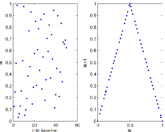
2.1Tent map
This type of map is characterized by a triangle shape fortk1with respect totk [19] and can be formulated as:
5 . 0 )
1 (
5 . 0
1
k k
k k
k
t t
t t
t
(3)
In this type of map, tk
0,1 the value we have will be tk1
0,1 too. The value of is suggested to be set to 2 [19]. Figure 1 shows characteristic of Tent map.1 (1 )
k c k k
t t t
k c
3.56, 4
0 t0 10{0, 0.25, 0.5, 0.75,1.0}
t
k
5
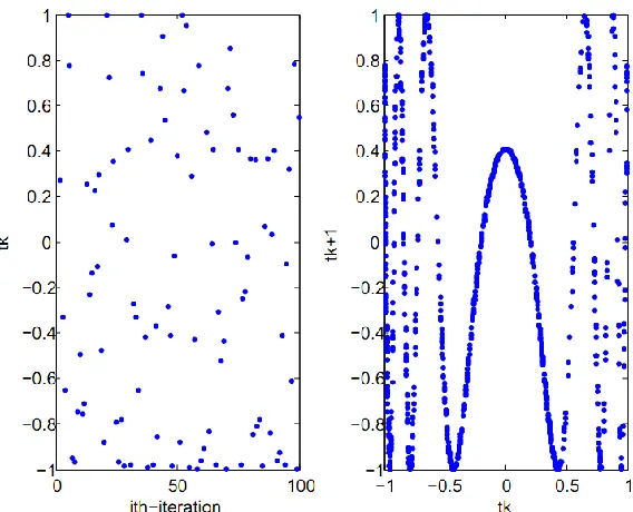
Figure 1. Plot of Tent one-dimensional map function: (left) time-series plot of the Tent map, (right) paired-plot between two consecutive chaos variables t.
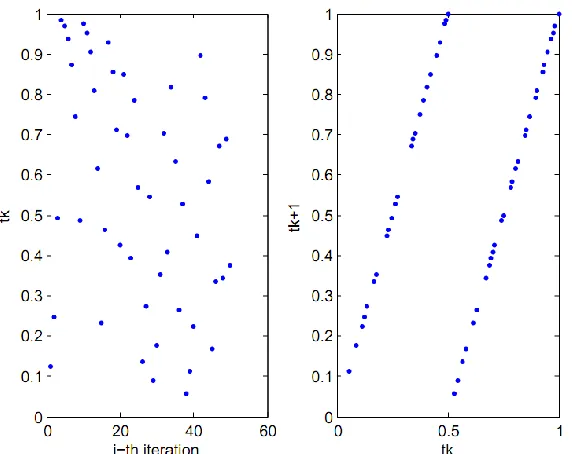
2.2Bernoulli shift map
The model comes from the effort to model the packages traffic in a network system [20]. The characteristic of this one-dimensional map is that in any successive iteration, considering two different initial valuest0andt0, the trajectories always diverge. The plot of this
one-dimensional map characteristic is presented in figure 2. The map can be formulated as:
1 1
) 1 (
1 0
1
1
k k
k k
k
t t
t t
t
(4)
6
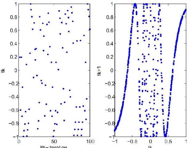
Figure 2. Plot of Bernoulli Shift map one-dimensional function: (left) time-series plot of the Bernoulli map, (right) paired-plot between two consecutive chaos variables t.
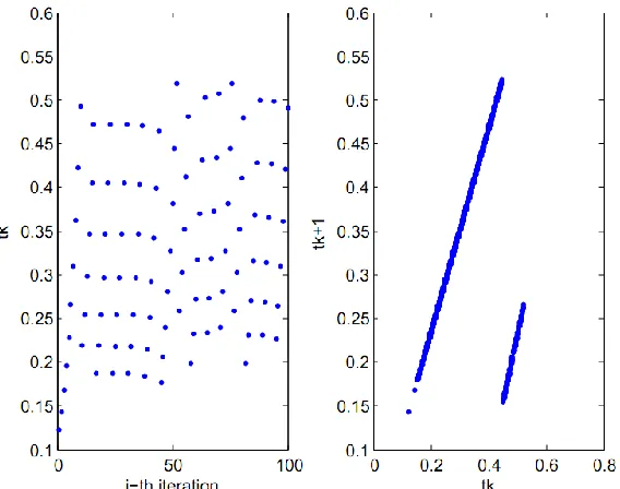
2.3Liebovitch map
Liebovitch and Tooth [23] proposed a one-dimensional map to model the kinetic activities of an ion channel. This map consists of three piece-wise linear segments which represent active, passive and switching region. The three segments have interval in
0,1 and they do not overlap. The Liebovitch one-dimensional map is formulated as:1
2
1 1
1
2 1
2 2
2
0
1 (1 ) 1
k k
k
k k
k k
t t d
d t
t d t d
d d
t d t
(5)
Where d1,d2 Î
( )
0,1 , d1<d2, 2
1 2 1
1 1 d
d d d
, and 2
2
1
2 1
2 1
1
1 d d d d
d
.
7
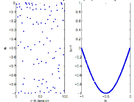
Figure 3. Plot of Liebovitch map one-dimensional function: (left) time-series plot of the Liebovitch map, (right) paired-plot between two consecutive chaos variables t.
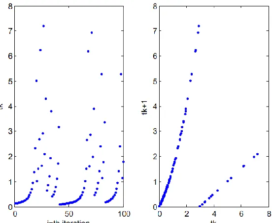
2.4Intermittency map
The one-dimensional intermittency map models the intermittency phenomenon, which is an irregular alternation of phases, in turbulence studies [24]. Figure 4 plots this type of one-dimensional map. A “sifting” phenomenon can be observed in its time series plot. This is the extension of Bernoulli map by introducing non-linear piece-wise functions. The two piece-wise functions represent passive and active period, for the first and second piece-wise function, respectively.
1 1
0
1
k k
k m
k k
k
t d d
d t
d t ct
t t
(6)
Where m
d d
8
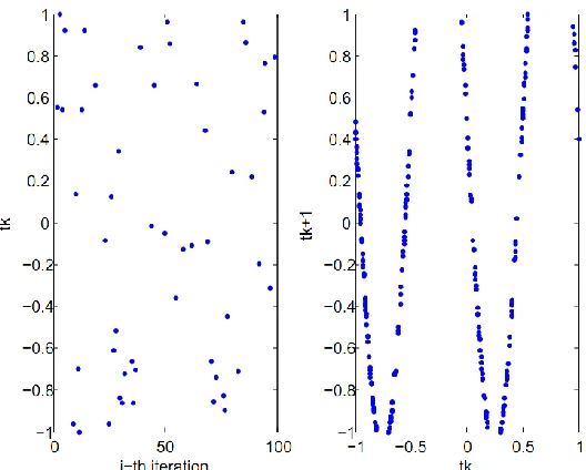
Figure 4. Plot of Intermittency map one-dimensional function: (left) time-series plot of the Intermittency map, (right) paired-plot between two consecutive chaos variables t.
2.5Chebyshev map
Characteristic of this one-dimensional map is that it has infinite collapse (high dynamic) within two symmetrical region of
1, 0
0,1
[20]. It means that the function is stable on the center point 0 and starts to collapse in the regions far from zero but in
1,1
. The Chebyshev map function is defined as:) cos cos( 1
1 k
k k t
t (7)
9
Figure 5. Plot of Chebyshev map one-dimensional function: (left) time-series plot of the Chebyshev map, (right) paired-plot between two consecutive chaos variables t.
2.6 ICMIC map
Iterative chaotic map with infinite collapse (ICMIC) is a one-dimensional map similar to the Chebyshev one. The difference between ICMIC and Chebyshev map is that in ICMIC the function response collapses (is unstable) at the center of two symmetrical region of
1, 0
0,1
. The regions far from the center area are stable area [20]. ICMIC map is defined as:) sin( 1
k k
t a
t (8)
10
Figure 6: Plot of ICMIC map one-dimensional function. (left) time-series plot of the ICMIC map, (right) paired-plot between two consecutive chaos variables t.
2.7 Gaussian map
This one dimensional map has the classical “bell shape” of the Gaussian distribution [21]. The map can be formulated as:
exp( )
2
1 n
k x
t (9)
11
Figure 7. Plot of Gaussian map one-dimensional function: (left) time-series plot of the Gaussian map, (right) paired-plot between two consecutive chaos variables t.
2.8Sine map
The shape of the sine one-dimensional map is qualitatively similar to the logistic map [22]. The formulation of this map is:
) sin( 4
1 k
k t
a
t (10)
Whereais an integer number and is selected equal to 2 [22]. This map is shown in figure 8.
Figure 8. Plot of sine map one-dimensional function: (left) time-series plot of the sine map, (right) paired-plot between two consecutive chaos variables t.
2.9Circle map
Physical motivation of this one-dimensional map the simulation of the behavior of driven mechanical rotors. Kolmogorov [22] first proposed this. Another physical relevance of this model is that it describes a model of phase looked loop in electronics. The circle map is formulated as:
) 2 sin( 2
1 k k
k t
K t
t
(11)
[image:11.612.166.445.198.411.2]12
Figure 9. Plot of circle map one-dimensional function: (left) time-series plot of the circle map, (right) paired-plot between two consecutive chaos variables t.
2.10 Algorithm complexity
For the combined Chaos-LM algorithm, a complexity analysis of the algorithm is applied to understand the relation between the growths of computational cost with respect to the number of input variables. In this case, the input variable is the number of points n to which the substitute geometry shall be fitted. One can observe that for each algorithm, CO and LM, there are two nested loops. In fact, these loops are not related to the number of points n, but only depends on a defined constant number. Only the procedure to calculate the objective function length relates to n is. As such, the computational growth can be stated as follow. Let the total order of the algorithms be f(n)n1 n2 nn2n, where subscript 1 and 2 correspond to algorithm 1 (CO) and 2 (LM), respectively. Hence, the algorithm efficiency is (n) since
) ( . ) ( , 0
0 0
0 and k n n f n k g n
n
so that f(n)n1n2 (n). Hence, the
complexity of the algorithm is linear with n.
3. Implementation and Performance comparison
13
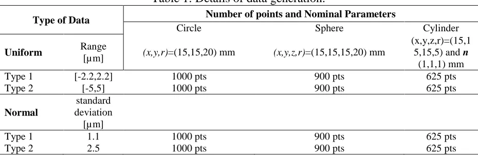
[image:13.612.74.539.274.428.2]The first approach generates points from some ideal geometry, which can be either a circle, a sphere or a cylinder. Noise is added which can be generated uniformly or normally distributed. Table 1 presents detail on the simulation. There are two levels of standard deviation considered for the data. Type 1 represents only the noise contribution from the instrument. Its sigma value is obtained from the instruments Maximum Permissible Error (MPE) [9-10] Type 2 instead simulates the contribution due to the part to part variability, including the instrument. Points generated by the second type represent a more realistic situation since an inspected part always contains some feature deviation from the nominal geometry [25]. Geometries will be generated both as full geometries and half geometries (e.g. a sphere and a hemisphere), giving rise to a total of six considered geometries. Reason to consider a half-geometry is that in many cases, points obtained by an instrument cannot cover the whole geometry due to, for example, surface accessibility problems, incomplete feature geometry, etc.
Table 1: Details of data generation.
Type of Data Number of points and Nominal Parameters
Circle Sphere Cylinder
Uniform Range
[µm] (x,y,r)=(15,15,20) mm (x,y,z,r)=(15,15,15,20) mm
(x,y,z,r)=(15,1 5,15,5) and n
(1,1,1) mm Type 1 [-2.2,2.2] 1000 pts 900 pts 625 pts Type 2 [-5,5] 1000 pts 900 pts 625 pts
Normal
standard deviation [µm]
Type 1 1.1 1000 pts 900 pts 625 pts Type 2 2.5 1000 pts 900 pts 625 pts
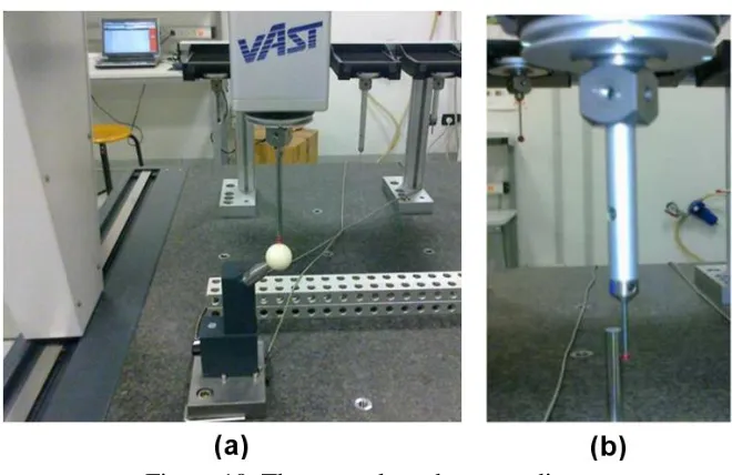
The second implementation and comparison is applied to points obtained from a series of real measurements by means of tactile coordinate measuring machine (CMM). Kawalec and Magdziak [26] reported comparison of methods to solve circle fitting problem by measuring a ring gauge as case study. There are two selected case studies for this real measurement approach: a reference ceramic sphere and an industrial cylinder. Figure 10 shows the measurement of the sphere and cylinder by tactile CMM.
As shown in figure 10(a), a calibrated ceramic sphere of a traceable tactile “ZEISS PRISMO” CMM with MPEE=2 µm+L/300 µm for stylus qualification was used with calibrated radius of
14
Figure 10. The two selected case studies:
(a) a ceramic sphere and (b) an industrial hardened steel cylinder.
The algorithm is implemented in MATLAB and run on an Intel Centrino Core 2 Duo 2.2 GHz. Center of circle and sphere is initialized by selecting the centroid of the cloud of points as initial guess. Moreover, the centroid is also the initial guess of a point on the axis of the cylinder. Initial estimation for radius is:
for the circle; (12)
for the sphere and cylinder (13)
Where 𝑟𝑜is initial radius estimation, 𝑥𝑜,𝑦𝑜,𝑧𝑜 are spatial coordinates of all the points. Only in the case of the cylinder, the initial guess for cosine direction of the axis is derived by fitting a 3D line to the point clouds.
Details of the performance improvement can be found in the previous paper [8]. A brief review of the results will be presented. From the results of previous study [8], the fitting performance has been improved by Chaos-LM algorithm. The performances considered are based on sum of square of residual error and speed to converge to an optimum solution. By Chaos-LM algorithm, the search can escape from local optima. The “local optima trap” is due to the Taylor approximation in the Gauss-Newton method. This approximation method highly depends on the non-linearity degree of the neighborhood. Since this approximation is usually applied up to the first term, the validity of this Taylor approximation decreases for higher non-linear function. Because of this, a “trapped” condition during the search process can occur.
0
(max min ) (max min ) 1
2 2
i i i i
x x y y
r
0
(max min ) (max min ) (max min ) 1
2 3
i i i i i i
x x y y z z
r
15
3.1 Performance evaluation of one-dimensional map functions
A previous paper of the authors of the present paper [8] has shown the improvement of the performance that can be obtained by applying Chaos-LM approach with a Logistic map. In this section, comparison of Chaos-LM algorithm performance with respect to different one-dimensional functions as chaotic motion generator of CO algorithm will be presented. The simulation data used for the comparison study is perturbed by noise applied to the nominal points. This noise is sampled from a uniform distribution in the range between -5 µm and 5 µm. This assumption includes the MPE (maximum permissible error) of a hypothetical CMM and the hypothetical part feature deviation. The complete results of the comparison, including both the norm of the residuals r and the CPU time, are presented in table 2. To compare the influence of different one-dimensional maps, an analysis of the variance (ANOVA) was carried out. Three replications (each replica is the mean value from 100 simulation runs) were carried out for each test. The treatments of the test are the continuous one-dimensional map. Identical to the previous section, response variables of the test is that the norm of the residual r and the CPU time. The test demonstrates that the map chosen significantly affect both r and CPU time, with the only exception of the CPU time for sphere fitting (figure 12(b)).
[image:15.612.73.545.555.709.2]The comparisons for full-geometries fitting are presented as bar chart in figures 11, 12, and 13, and for half-geometries in figures 14, 15, and 16. From these figures, one can observe that, in general, the logistic-map is the most effective to solve the optimization problem in terms of r , with some compromises of having higher computational time in certain cases. For example, in the case of half-circle fitting, the logistic map provides the best solution, but the computation time is significantly higher with respect to all the others. In full-circle fitting (figure 11), Liebovitch and Intermittency chaos generation give the worst solution while for full-cylinder fitting (figure 13), Bernoulli Shift and Sine chaos generator give the worst solution. A solution in general similar is observed in the case of full-sphere fitting (figure 12). Higher variation in results is observed in the case of half-geometries compared to the full geometries. Liebovitch and Intermittency generator give the worst results for half-sphere and half-cylinder. Bernoulli Shift, Sine, and Circle generator gives the worst results of half-circle fitting. Table 4 gives the detail results of the comparison runs.
Table 2: Complete result of several types of one-dimensional map. Random
Error Type (um)
Type of One-Dimensional
Map
Full-Geometries Chaos and Levenberg-Marquardt Algorithm
Circle Sphere Cylinder
||r|| (µ±3σ) CPU time (µ±3σ) ||r|| (µ±3σ) CPU time (µ±3σ) ||r|| (µ±3σ) CPU time (µ±3σ)
U[-5,5]
Logistic 3,3562 ±4,4067 0,5551 ±0,0308 6,2199 ±0,4602 0,5628 ±0,1088 5,7994 ±2,9641 0,6706 ±0,0515
Tent 3,8789
±1,3553 0,5400 ±0,0282 6,2625 ±0,5551 0,4987 ±0,0856 5,0455 ±1,9903 0,7874 ±0,1155
Bernoulli Shift 28,4587 ±10,1690 0,4947 ±0,0941 7,5839 ±1,5888 0,6106 ±0,3284 88,752 ±3,2902 0,7665 ±0,0997
16
Intermittency 92,9567 ±5,6253 ±0,1139 0,4994 ±0,8001 7,1161 ±0,0266 0,4675 ±0,4035 3,3571 ±0,0443 0,7795
Chebyschev ±10,6941 37,4017 ±0,0794 0,5637 ±0,7605 6,975 ±0,0247 0,5527 ±0,4954 3,2422 ±0,0703 0,7885
Gaussian 3,8776 ±1,5751 0,5948 ±0,1065 6,3682 ±0,8676 0,5628 ±0,1068 2,9529 ±0,0444 0,7823 ±0,0527
Sine ±1,0583 2,8379 ±0,0896 0,4947 ±1,2561 6,6963 ±0,0295 0,5531 ±11,0938 81,9015 ±0,0991 0,8223
ICMIC 27,3192 ±10,6311 0,4862 ±0,0732 6,9606 ±0,8579 0,5782 ±0,1159 2,9676 ±1,1675 0,8172 ±0,0383
Circle 22,3999 ±10,0398 0,5216 ±0,0947 7,4993 ±1,7130 0,5840 ±0,1275 88,5412 ±4,1864 0,785 ±0,0915 Random Error Type (um)
Type of One-Dimensional
Map
Half-geometries Chaos and Levenberg-Marquardt Algorithm
Circle Sphere Cylinder
||r|| (µ±3σ) CPU time (µ±3σ) ||r|| (µ±3σ) CPU time (µ±3σ) ||r|| (µ±3σ) CPU time (µ±3σ)
U[-5,5]
Logistic 15,9923 ±12,0558 1,2212 ±0,1456 9,2163 ±6,3610 0,413 ±0,0247 18,7634 ±3,0584 1,2185 ±0,1001
Tent 99,9067
±10,5034 0,4945 ±0,0642 10,8683 ±2,3928 0,458 ±0,0601 18,8646 ±1,6585 1,6603 ±0,2450
Bernoulli Shift 116,6437 ±6,0842 0,5704 ±0,1080 20,1410 ±10,4110 0,4742 ±0,0704 39,7236 ±3,7368 1,7059 ±0,2628
Liebovitch 100,4388 ±12,9591 0,4843 ±0,0373 43,1376 ±3,7162 0,4667 ±0,0795 18,8829 ±1,5393 1,6815 ±0,1123
Intermittency 48,8010 ±6,9925 0,5731 ±0,0601 43,1131 ±4,7619 0,5632 ±0,0349 18,9943 ±1,7687 1,6443 ±0,1796
Chebyschev 22,7672 ±10,8399 0,5440 ±0,0267 27,5289 ±15,9982 0,5622 ±0,0382 18,8082 ±2,0556 1,6513 ±0,1084
Gaussian 60,9419 ±10,9246 0,5017 ±0,1493 11,5014 ±10,2587 0,5802 ±0,0749 18,9913 ±1,2906 1,5953 ±0,2921
Sine 115,0962 ±9,9298 0,4721 ±0,0462 20,0862 ±10,0986 0,5693 ±0,0880 28,5602 ±12,6451 1,5441 ±0,1390
ICMIC 15,2252 ±5,8807 0,5587 ±0,0316 28,6431 ±14,0605 0,4731 ±0,0362 19,142 ±2,5265 1,5227 ±0,3441
17
Figure 11. Comparison of type of one-dimensional map for Chaos-LM method for full circle point cloud fitting: (a) Norm of residual, (b) CPU time.
[image:17.612.78.538.307.477.2]18
[image:18.612.77.540.293.465.2]Figure 13. Comparison of type of one-dimensional map for Chaos-LM method for full cylinder point cloud fitting: (a) Norm of residual, (b) CPU time.
Figure 14. Comparison of type of one-dimensional map for Chaos-LM method for half circle point cloud fitting: (a) Norm of residual, (b) CPU time.
[image:18.612.83.539.509.684.2]19
Figure 16. Comparison of type of one-dimensional map for Chaos-LM method for half cylinder point cloud fitting: (a) Norm of residual, (b) CPU time.
In addition, the performance comparison among one-dimensional map of CO method is also carried out on real measurement data. The results are shown in figures 17, 18, and 19 for real case studies of sphere measurement with low-density points, with high-density points and industrial cylinder measurement, respectively. Table 3 presents the detailed results of the comparison study. From these graphs, one can observe that the comparisons of the one-dimensional map performance are similar to those proposed earlier. Logistic map, Liebovitch map and Gaussian map obtained the best result for the norm of residual in the case of both the sphere fitting from low and high-density points. Instead, in the case of industrial cylinder fitting, Tent, Intermittency and Chebyshev map give the least norm of residual. Logistic map does not perform well only in this case. This could be caused by small number of points to fit compared to other case studies. About the CPU time needed to fit the data, there is no significant difference among the different one-dimensional map functions.
Table 3: Detail results of comparison of one-dimensional map for real measurement case study.
Random Error Type
Type of One-Dimensional Map
Chaos and Levenberg-Marquardt Algorithm
[image:19.612.73.570.484.699.2]Sphere Low Density Sphere High Density Industrial Cylinder
||r|| (µ±3σ) CPU time (µ±3σ) (µ±3σ) ||r||
CPU time (µ±3σ)
||r|| (µ±3σ) CPU time (µ±3σ)
U [-0.005,0.005]
Logistic 0,5139 ±0,5044 0,4991 ±1,961 2,2776 ±1,882 3,8707 ±0,33 2,1981 ±0,4822 8,4489 ±2,3731
Tent 1,2014 ±0,8465 0,4683 ±0,0221 4,2608 ±2,5093 4,0577 ±0,025 0,4197 ±0,7331 8,2408 ±1,5865
Bernouli Shift 17,8537 ±0,02 0,46823 ±0,024 57,3112 ±1,8702 4,0531 ±0,037 3,6392 ±0,0079 6,9392 ±1,99
Liebovitch 0,7122 ±0,5861 0,4629 ±0,0167 1,9955 ±0,6037 4,0732 ±0,052 3,3185 ±1,6297 8,3943 ±0,2994
Intermittency 3,1645 ±0,9661 0,4736 ±0,0385 7,8977 ±3,2939 4,358 ±0,9656 0,3209 ±0,6761 8,5420 ±0,1524
20
Gausian 0,5855 ±0,4368
0,4687 ±0,0222
1,7241 ±2,0967
5,2739 ±2,9522
3,6351 ±0,02
8,514 ±0,4319
Sine 17,5325 ±0,6418
0,4642 ±0,082
55,2934 ±6,6626
4,6047 ±2,7276
3,6392 ±0,02
8,9919 ±1,9286
ICMIC 17,73143 ±0,1382
0,4676 ±0,0282
2,0303 ±0,5039
5,0282 ±4,7533
0,455 ±0,05
8,5241 ±0,0868
Circle 17,8149 ±0,1784
0,4629 ±0,072
57,3171 ±0,7026
4,1288 ±0,127
3,6391 ±0,02
[image:20.612.68.554.70.382.2]9,0029 ±1,313
Figure 17. Comparison of type of Chaos one-dimensional map for sphere measurement with low density points (312 points): (a) Norm of residual, (b) CPU time.
[image:20.612.80.539.431.597.2]21
Figure 19. Comparison of type of Chaos one-dimensional map for industrial cylinder measurement (190 points): (a) Norm of residual, (b) CPU time.
4. Concluding Remarks
In this article, the problem of fitting non-liner geometries has been discussed. This fitting procedure is critical in the whole chain of dimensional metrology. The reason is that many product quality inspections are realized by means of dimensional quality inspection. Modern metrology instruments can capture high density clouds of points in short time. Hence, this fitting problem becomes more and more relevant. Three non-linear geometries are considered in this work, due to their diffused use in applications such as metrological calibration and mechanical assembly: circle, sphere and cylinder. Both cases of fitting full- and half-geometries are addressed. It has been shown that a performance improvement of the fitting results from simulated and real measurement data can be obtained by combining chaos optimization and LM algorithm compared to a single LM algorithm. The LM method is in many cases trapped and early converged during the optimization process, in particular in the case of half-geometries fitting. In this situation, no improvement of the result can be obtained by increasing the number of iterations. Comparison among various type of one-dimensional map, which determine the chaos motion, is presented as well. A total of 10 one-dimensional map functions are considered. This comparison study points out that, in general, the logistic map function performs the best in almost all situations compare to other type of one-dimensional maps. The future direction of this work is the identification of the link between the non-linear problem and chaos properties such that an adaptive region bounding and chaotic motion generation can be better determined. This perspective is motivated by the development of specific method for sphericity measurement [27]. In this paper, they show that a specific method can be developed for a specific fitting problem (in this case a sphere fitting problem). With relation with chaos algorithm, a specific development of the algorithm for a specific fitting problem may improve the performance for the specific developed case over the general chaos algorithm for all type of non-linear geometric fitting problem.
Acknowledgements
22
(Italy), CUP: D81J10000220005 and AMALA – Advanced Manufacturing LAboratory, funded by Politecnico di Milano (Italy), CUP: D46D13000540005.
References
[1] Kunzmann H, Pfeifer T, Schmitt R, Schwenke H, Weckenmann A 2005 Productive Metrology-Adding Value to Manufacture CIRP Ann. Manuf. Techn. 54(2) 155 – 168.
[2] Pereira P H 2012 Cartesian Coordinate Measuring Machines, in Hocken R. J., Pereira, P. H (Eds), Coordinate Measuring Machines and Systems 2nd ed, (Florida:CRC Press) 57-79.
[3] Morse E 2012 Operating a Coordinate Measuring Machine, in Hocken R. J., Pereira, P. H (Eds), Coordinate Measuring Machines and Systems 2nd ed, (Florida:CRC Press) 81-91.
[4] Wilhelm R G, Hocken R, Schwenke H 2001 Task Specific Uncertainty in Coordinate Measurement CIRP Ann. Manuf. Techn. 50(2) 553-563.
[5] Muralikrishnan B, Raja J. 2009 Computational surface and roundness metrology (New York: Springer).
[6] Hoppe H, DeRose T, Duchamp T, McDonald J, Stuetzle W 1992 Surface reconstruction from unorganized points ACM 26(2) 71-78.
[7] Moroni G, Petrò S, Tolio T 2011 Early cost estimation for tolerance verification CIRP Ann. Manuf. Techn. 60(1) 195-198.
[8] Moroni G, Syam W P, Petro S. 2014 Performance improvement for optimization of the non-linear geometric fitting problem in manufacturing metrology Measurement Science and Technology 25 085008.
[9] ISO 10360-4:2010 2010 Acceptance and re-verification test for coordinate measuring machines: CMM used in scanning measuring mode.
[10] ISO 10360-5:2010 2010 Acceptance and re-verification test for coordinate measuring machines: CMM using single and multiple styluses contacting probing system.
[11] Moroni G, Petrò S, Syam W P. 2014 Four-axis micro measuring systems performance verification CIRP Annals-Manufacturing Technology Vol. 63 (1), 485-488.
[12] Moroni G, Syam W P, Petrò S. 2015 On Performance Verification of Simultaneous 4-axis 3D Geometric Optical Instrument LAMDAMAP XI, 17-18 March 2015, Huddershfield, UK.
23
[14] Marquardt D W 1963 An Algorithm for Least-Squares Estimation of Non-linear Parameters, J. Soc. Ind. Appl. Math. 11(2) 431-441.
[15] Nash J C 1979 Compact Numerical Methods for Computers Linear Algebra and Function Minimization (Bristol: Adam Higler Ltd).
[16] Rardin R L 2006 Optimization in Operation Research (New York: Addison-Wesley).
[17] Janecki D, Stepien K, Adamczak S 2010 Problems of measurement of barrel- and saddle-shaped elements using the radial method Measurement 43 659-663.
[18] E. Ott, Chaos in Dynamical Systems, Cambridge University Press, Cambridge, UK, 2002.
[19] A. Erramilli, R.P. Singh, P. Pruthi, Modeling packet traffic with chaotic maps, Royal Institute of Technology, ISRN KTH/IT/R-94/18-SE, Stockholm-Kista, Sweden, August 1994.
[20] D. He, C. He, L. Jiang, H. Zhu, G. Hu. 2001. Chaotic characteristic of a one-dimensional iterative map with infinite collapses, IEEETransactions on Circuits and Systems, Vol. 48 (7) 1076-1085.
[21] M. Bucolo, R. Caponetto, L. Fortuna, M. Frasca, A. Rizzo. 2002. Does chaos work better than noise?, IEEE Circuits and Systems Magazine, Vol. 2 (3) 4-19.
[22] R.L. Devaney, An Introduction to Chaotic Dynamical Systems, Addison-Wesley, USA, 2003.
[23] Liebovitch LS and Tooth TI. 1990. Ion Channel Kinnetics: Random or Deterministic Process?. Biophysical Journal, Vol. 57, 317a.
[24] Schuster, H. G. 2005. Deterministic Chaos: An Introduction, 2nd Ed. Wiley-VCH Verlag GmbH: Germany.
[25] Kruth J P, Van Gestel N, Bleys P, Welkenhuyzen F. 2009 Uncertainty determination for CMMs by Monte Carlo simulation integrating feature form deviations CIRP Ann. Manuf. Techn. 58(1) 463-466.
[26] Kawalec A and Magdziak M 2012 Usability assessment of selected method of optimization for some measurement task in coordinate measurement technique Measurement 45 2330-2338.
[27] Janecki D, Stepien K, Adamczak S 2016 Sphericity measurements by the radial method: I. Mathematical fundamentals Measurement Science and Technology, Vol. 27, No. 1, pp. 015005.
24
[29] Luo Y Z, Tang G J, Zhou N L 2008 Hybrid approach for solving systems of nonlinear equations using chaos optimization and quasi-Newton method Applied Soft Computing 8(2) 1068-1073.