Finite control set and modulated model predictive flux and current control for induction motor drives

Finite Control Set and Modulated Model Predictive

Flux and Current Control for Induction Motor Drives

S. A. Odhano, A. Formentini, P. Zanchetta Department of Electrical and Electronic Engineering

The University of Nottingham Nottingham, NG7 2RD, United Kingdom

R. Bojoi, A. Tenconi Department of Energy

Politecnico di Torino Torino, 10129, Italy

Abstract — The paper presents a new implementation of direct flux and current vector control of an induction motor drive using the techniques of model predictive control. The advantages offered by predictive control are used to enhance the dynamics of direct flux vector control. To minimize the problems of variable switching frequency inherent to finite control set predictive control, an alternative approach using pulse width modulation is studied for command execution as occurs in the so-called modulated model predictive control. A comparison between finite control set and modulated model predictive control is presented and the results are also compared with the control implementation through traditional proportional-integral regulators to highlight the advantages and drawbacks of predictive control based strategies. Apart from a greater harmonic content in stator currents, the predictive control can offers control dynamics comparable with proportional-integral control while maintaining immunity against machine parameter variations and excluding the need for controller tuning.

Keywords—predictive control, state estimation, signal sampling, variable speed drives, induction motors, machine control, mathematical model, pulse width modulation converters

I. INTRODUCTION

After its conception in the early ‘60s and successful implementation for industrial process control ever since, the model predictive control [1-5] has gained popularity in the recent past for its application in power electronics control [6-8, 19] that has opened a host of possibilities for the control of power converters. Although this control type’s use has majorly focused on converter control, the trend of its application for variable speed drives control is also on the rise [8-18].

Model predictive control’s salient features include faster dynamics, simpler treatment of actuator constraints, allowing multivariable control with least complexity, permitting easier inclusion of non-linearities in the model, adaptability for fitting specific applications, ease of implementation and extension. The above advantages, however, do incur a cost in terms of greater computational power requirements [3], with respect to traditional control strategies (e.g. linear controllers), as well as the dependence of control performance on the quality/accuracy of the plant/process model. In power electronic systems, the model predictive control, due to its inherent nature resembling a hysteresis control, requires variable switching frequency operation that entails greater ripple in controlled variables’

waveforms. Some of these disadvantages can be circumvented by mathematical simplifications and limiting the control and/or prediction horizons, obviously compromising on the overall control performance.

Current research trends on the application of model predictive control (MPC) in power electronic systems focus on the following four macro areas: grid-connected converters, power converters supplying R-L loads, inverters with L-C output filters, and high performance motor drives [6]. In the area of motor drives, MPC has been very successfully employed for predictive torque control (PTC) [9, 10, 13, 14] and predictive current control (PCC) [13], and predictive flux control (PFC) [11] and speed control [15] of induction motor drives. The research extended the use of MPC to sensorless [14, 16, 17] as well as fault tolerant [12] induction motor drives. The MPC’s application range is not limited to three-phase applications but has also encompassed multithree-phase induction machine topologies [12].

Of the many works found in the literature on the subject of MPC application in electric drives, those most closely related to this work are [9, 10, 11, 13]. In [9], the authors have proposed predictive torque control for a multilevel-inverter-supplied induction motor drive. The multilevel strategy considerably reduces the torque and flux ripple that is naturally present in the direct stator variable control schemes (with no integral smoothening effect of a PI controller). However, the increased hardware complexity cannot be overlooked. A modified model predictive torque and flux control strategy is proposed in [10] that uses the active vectors’ duty cycle to ensure fixed switching frequency operation. The duty cycles of the active vectors are optimized through torque dead beat control. As in other works dealing with torque and flux predictive control, in this work the selection criteria of weighting factor to assign right priority to torque and flux errors is a matter of extensive simulation and experimental verification. The stator flux’s model predictive control strategy of [11] is a sequel of [10] and uses the same duty cycle optimization strategy, here called switching instant optimization, to achieve flux control.

A performance comparison of PTC and PCC is presented in [13] with experimental verification. The torque and current predictive controls are shown to have comparable dynamic performance but the predictive torque control has lower ripple than its current control counterpart. In open-loop torque control

mode, both the methods have non-zero steady state error. The PCC is shown to be sensitive to errors in stator resistance and the PTC is vulnerable to errors in magnetizing inductance.

In this paper, the MPC is adopted for another control strategy of induction motor (IM) drive that has recently been developed, the direct flux vector control (DFVC) [20-22]. This control scheme combines the advantages of direct flux and torque control and the current vector control. The control strategy is first briefly described and then expressions are derived for use with predictive control algorithms. Simulation results with a non-linear induction machine model; are given using the finite control set MPC (FCS-MPC) and modulated MPC (M2_{PC) for flux and current control. The results are}

compared with the traditional proportional-integral (PI) regulators based approach and conclusions are drawn by performing a cost-benefit analysis.

II. MODEL FOR FLUX AND CURRENT CONTROL

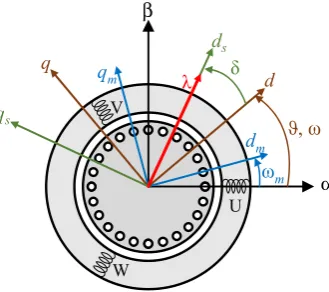
[image:2.595.358.523.54.200.2]

The direct flux and current vector control (DFCVC) strategy is implemented in the stator flux-oriented reference frame with the ds-axis aligned with stator flux vector (λ) as shown in Fig. 1. The other reference frames shown in the figure are the rotor flux frame (d, q), the rotor mechanical frame (dm, qm) and the stationary (α, β) frame. The induction motor’s dynamic equations in the stator flux-oriented (ds, qs) reference frame are given by:

dqs dqs dqs s dqs dt d j dt d i R

v _λ

    _ω+ δ +

λ +

= (1)

where Rs is the stator resistance, ω is the synchronous speed in rad/s and δ is the load angle, while

v

_dqs

,

i

_dqs

,

_λ

_dqsare the stator voltage, current and flux vectors, respectively. The subscript ‘s’ refers to the stator flux-frame for which the flux vector is defined as:

λ = + λ = λ + λ =

λdqs ds j qs j0 (2)

The stator and rotor flux linkages of an IM are related to current as per (3) and (4).

In (α, β) frame λs=krλr+σLsis (3)

In (dm, qm) frame r r r krRris

dt d + λ τ − =

λ −1 ₍₄₎

where σ is the total leakage factor and Ls is the total stator inductance; kr = Lr/Lm is the rotor coupling factor with Lr and

Lm being the rotor and magnetizing inductance, respectively, and, finally, τr defined as τr = Lr/Rr is the rotor time constant with Rr as the rotor resistance. Equations (3) and (4) are the basis for the IM flux observer.

α β U V W dm

q_{m d}

ωm

ϑ, ω

ds q

qs

δ

λ

Fig. 1. Reference frames definition for DFCVC.

The instantaneous electromagnetic torque of the machine is given by:

qs

i p

T = λ

2

3 ₍₅₎

Transforming (1) to state-space notation, after substituting (2), yields:               λ − − +       δ λ       ω − =               δ λ qs s qs ds s ds i R v i R v dt d dt d 0 0 0 (6)

It can be observed that the flux dynamics solely depend on the ds-axis voltage command thus a fast flux control can be achieved by acting on vds. Equation (6) also suggests that the control of state variable δ through qs-axis voltage is not completely independent of λ; the appearing of λ in the denominator of the control action for δ further complicates the control scheme and the control design is not straightforward. Moreover, the torque expression (5) hints at having the qs-axis current as the other state variable for better torque control. It is possible to transform the second state equation to have iqs as the other state variable; a detailed derivation is given in [23], here we report the final expression for brevity.

(

−ω λ

)

+ σ ω + ′ − =

σ qs slip s ds qs m

qs

s _dt Ri L i v

di

L (7)

[image:2.595.362.506.342.406.2]

III. MODEL PREDICTIVE CONTROL FORMULATION The state equations defined in (8) can be converted to discrete-time equivalents using Euler’s approximation for the derivative terms as:

(

k+

) ( )

=λ k +Ts

(

vds

( )

k −Rsids

( )

k

)

λ 1 (9)

(

)

( )

( )

( )

k T i

( )

k v L T k i L T R k L T k i ds slip s qs s s sq s s s s m sq ω + σ + +       σ ′ − + λ σ ω − =

+1 1

(10)

where Ts is the sample time for discretization.

Equations (9) and (10) would serve as one-step-ahead predictors for the state variables (λ and isq). However, to compensate for the delay between command generation and its effective realization, [24] suggests two-step-ahead prediction of the states. In our case, one state is the stator flux (λ) which is given by the flux-observer that already serves as a one-step-ahead predictor because the flux-observer’s inputs are the voltage commands applied at previous switching and sampling instant, if switching is synchronized with sampling. Thus, (9) is shifted one step forward in time. We use two-step-ahead prediction of [24] only for the current (isq) state variable, using (11).

(

)

(

)

(

)

(

k

)

T i

( )

k v L T k i L T R k L T k i ds slip s qs s s sq s s s s m sq ω + + σ + + +       σ ′ − + + λ σ ω − = + 1 1 1 1 2 (11)

[image:3.595.383.479.176.373.2]

To further improve isq prediction accuracy in (11), we use the prediction of stator flux λ(k+2) since it precedes isq prediction and does not need isq for its computation (cf. eq. (9)). Fig. 2 shows the sequence in which (9), (10) and (11) are applied for state estimation.

k+1

kT_s k

( ) ( ) ( )

( 1)

~ (10) Eq. meas. current 1 ~ , : observer flux +  + + λ  αβ αβ k i k k i k v sq ( )

( 2) min( ) ( 1)

[image:3.595.63.291.381.435.2] [image:3.595.38.286.511.552.2]

~ (11) Eq. 2 ~ (9) Eq. +       +  + λ  k v g k i k c sq

Fig. 2. State variable prediction and control action calculation sequence.

The cost function (gc) to be minimized to achieve predictive control is given in terms of reference and actual/predicted magnitudes of the state variables (λ and isq) given in (12).

p sq sq p

c i i

g = λ∗−λ + ∗ − ₍₁₂₎

Where superscript ‘*’ is used for imposed reference and ‘p’ stands for predicted value. In order to assign equal weight to the two dimensionally different state variables, the per-unit values are used as a rather simplistic way of dealing with a complex problem. For torque and flux predictive control found

in the literature, the tuning of weights assigned to each variable is still a matter of research and no empirical tuning method exists to date [10, 18, 25]. The tuning of weights for flux and current state variables used here may also be treated in depth in a future work.

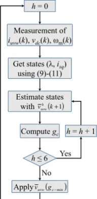
The flowchart of Fig. 3 gives the sequence of operations for direct flux and current vector predictive control of an induction machine. When the cost function is evaluated for all the possible voltage vectors, the vector that corresponds to minimum value of cost function (gc-min) is applied.

Measurement of iuvw(k), vdc(k), ωm(k)

Get states (λ, isq)

using (9)-(11)

Estimate states withvh (k+1)

uvw

Compute g_c

Apply

h≤ 6 Yes

No

h=h+ 1 h= 0

( cmin) uvwg

v ₋

Fig. 3. Process flow chart for predictive flux and current control.

IV. FCS-MPC AND M2_PC

The finite control set (FCS) MPC with a three-phase two-level power electronic converter acts within a finite set of possibilities, which are the inverter switching states consisting of six active vectors and two zero vectors. The two zero vectors are identical, and therefore redundant, so only one of them is considered as a possible command signal to reduce the number of calculations per execution cycle. As shown in the flowchart above, once the cost function is minimized, the inverter switching state that corresponds to minimum value of gc is applied during the next switching instant. As the available switching states are limited and, in the absence of a modulator, the converter must apply a given state for the entire switching period that not only causes a greater ripple in the controlled variables and may also entail a variable (albeit reduced) switching frequency thus degrading the performance of MPC with respect to its competitors that use modulators (such as the linear controllers). Besides, an increased switching frequency will result in greater commutation losses in the power electronic switches. However, this disadvantage should not be overstated without looking at the average switching frequency with FCS-MPC that can be significantly lower than the fixed switching frequency usually used with the modulator-based command generation.

modulation (PWM or SVM) is referred to as the modulated MPC (M2_{PC). It can be argued that the modulated MPC has}

infinite control set as the available choice thus the cost function minimization becomes an optimization problem, however, by limiting the output to six active and one zero vectors, the problem is transformed back to a finite control set one thus avoiding the use of computationally demanding optimization algorithms. The flowchart of Fig. 3 for state estimation and cost function evaluation remains unchanged except the last step where vuvw(gc-min) is passed to a modulator that applies the

corresponding inverter switching states with a fixed switching frequency while complementing the remaining switching period with one of the two zero vectors that requires minimum switching operations to minimize commutation losses.

The use of M2_{PC in our case of direct flux control brings an}

added benefit, over FCS-MPC, as it allows limiting the ds-axis voltage that is helpful in containing the ds-axis current to a safe value since it is not feedback controlled. Noting from (8) that a fast flux control would require the entire available phase voltage being applied along the ds-axis, it may cause the machine phase current (limited only by stator resistance) to reach amplitudes that could trigger overcurrent protection. This feature is particularly helpful when working with low resistance machines.

V. RESULTS AND DISCUSSION

The block diagram for the implementation of DFCVC strategy through MPC is shown in Fig. 4. The scheme is shown for speed control but it can equally be used in torque control mode. The MPC block can either be FCS-MPC or M2_{PC, the}

output of the block is in terms of switching signals which is true for FCS case but, for the modulated alternative of MPC, the block’s output is PWM modulated. The block named (λ, isq) = f(vdc, ωm, T*) contains the operating point dependent functions such as flux-weakening, maximum torque per ampere (MTPA), and maximum torque per volt (MTPV) characteristics of the machine defined as per [21, 22]. The flux-observer and field orientation block is expanded in Fig. 5 where DT stands for dead-time compensation and g is the flux observer’s crossover frequency (in rad/s) between stator and rotor equation based estimation. The flux observer is implemented using (3) and (4). The block called ‘Magnetic Model’ contains the machine’s saturation characteristic as well as the rotor equation model (4).

Fig. 6 gives results for the scheme of Fig. 4 being used as FCS-MPC of flux and current vector control. Note that the machine is pre-excited with a ramp to keep the excitation current in check. To give a fair comparison, all the schemes are subjected to this flux ramp. Furthermore, the sampling frequency is limited to 10 kHz for FCS-MPC to compare all the three strategies under similar conditions, since M2_{PC and}

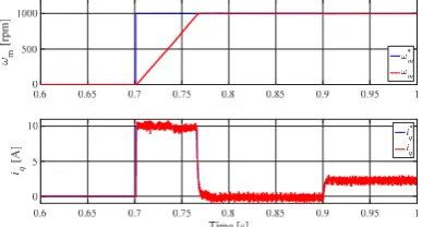
PI-based implementation have 10 kHz switching and sampling frequency. As can be seen in Fig. 6, the excitation current is not pretty clean which can be expected of the FCS-MPC that applies a given switching state for the entire switching period. In Fig. 7, the speed step response with FCS-MPC is shown. The speed loop bandwidth is 16 Hz in all three cases. The

qs-axis current is saturated to 10 A to limit the total phase current, this limitation is equally applied to all three control

schemes for fair comparison. At t = 0.9s a load torque equal to 50% of the machine’s rated torque is applied.

[image:4.595.312.554.180.256.2]

The results for modulated MPC (M2_{PC) are presented in}

Fig. 8 and 9 for flux and speed (and current) control dynamics, respectively. The ds-axis voltage is limited to contain the

ds-axis current. This results in deteriorating performance of flux loop at the instant when the speed step is applied. The benefits of M2_{PC can be seen in terms of contained distortions}

in id. The speed response of Fig. 9 and the corresponding

qs-axis current response are comparable with those of Fig. 7.

* m

ω PI T* (λ, isq) =

f (vdc, ωm, T*) MPC

vdc

+ −

IM

vdc uvw

i

ϑm

Δuvw

λˆ Speed compute

ϑm Flux Obs.,

field orient. dq

i vdq –

[image:4.595.318.542.292.420.2]

vdc

Fig. 4. Block diagram for model predictive direct flux and current vector control for a speed controlled IM drive.



m

j

e−ϑ Magnetic ejϑm model

αβ

i

dt

v_αβ

r

αβ

λ

~

r

αβ

λˆ +

ϑm

x , x ∠ ϑˆ_s

λˆ

uvw

i uvw_αβ

vdc · uvw_αβ

– –

Δuvw

DT Rs

αβ v

–

g

–

+

s

j

e−ϑ

dq

i

s

j

e−ϑ vdq uvw

v

αβ

i

σLs

–

s

αβ

λ ₊

[image:4.595.333.533.442.553.2]

1/kr

[image:4.595.337.531.581.685.2]

Fig. 5. Details of the flux observer and field orientation block of Fig. 4.

Fig. 6. Flux loop dynamics for FCS-MPC. Load torque is applied at t = 0.9s. Top axis: reference and actual stator flux, bottom axis: ds-axis current.

[image:5.595.317.547.51.174.2] [image:5.595.50.279.53.183.2]

Fig. 8. Flux control performance of M2_{PC. Load is applied at t = 0.9s.} Top axis: reference and actual stator flux, bottom axis: ds-axis current.

Fig. 9. Speed response and current control for M2_{PC with load torque being} applied at t = 0.9s. Top axis: reference and actual speed, bottom axis: commanded and real qs-axis current.

Finally, the control performance with the PI-based implementation is shown in Fig. 10 and 11. The closed-loop bandwidth of the flux and current control is set as 791 Hz and 1080 Hz, respectively. The flux and current loops’ performance is decisively superior with respect to the FCS-MPC. The M2_PC

is bettered in terms of flux loop while the current loop dynamics are comparable. However, M2_{PC enjoys greater}

immunity to machine parameter variations compared to PI regulators as the obtained bandwidth of the PI controllers varies with parameters. Furthermore, the MPC does not require tuning of PI controller gains. As with other applications of MPC in power electronics and drives [6], analytical expressions cannot be derived to prove MPC’s robustness against parameter variations. Simulations and experiments performed with detuned parameters could be used to ascertain the degree of immunity to parameter deviations.

[image:5.595.42.283.209.339.2]

Fig. 10.Control dynamics of flux loop with PI regulator. Load torque is applied at t = 0.9s. Top axis: reference and actual stator flux, bottom axis: ds-axis current.

Fig. 11.Speed and current loop dynamics for PI regulators based implementation. Load rejection capability is verified by applying load torque at t = 0.9s. Top axis: speed step reference and rotor mechanical speed, bottom axis: qs-axis current’s reference and actual values.

A slight increase in the ds-axis current is observed in all three cases when the load torque is applied. This is due to the fact that, with the application of qs-axis current, the machine saturates that requires greater ds-axis current to maintain stator flux at the desired level.

Moreover, a comparison in terms of stator phase currents is shown in Fig. 12 for the three control implementations. The FCS-MPC draws distorted current principally due to ds-axis noise (cf. Fig. 6). The M2_{PC and PI-based control strategies}

have comparable current waveforms. Furthermore, for low resistance machines, the peak phase current can be controlled in the latter two cases by limiting the ds-axis voltage reference applied to the modulator which is not possible with FCS-MPC.

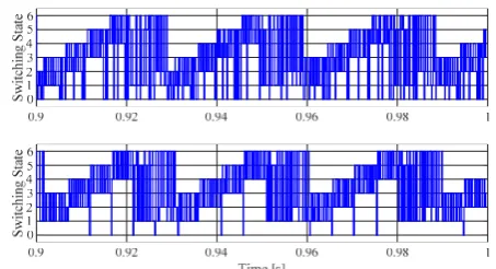
In order to compare the FCS-MPC with its modulated counterpart (M2_{PC), Fig. 13 gives the converter switching}

Fig. 12.Stator phase-U current for the three control implementations. Top: FCS-MPC, centre: M2_{PC, bottom: PI.}

Fig. 13.Inverter switching states corresponding to gc-min for model predictive

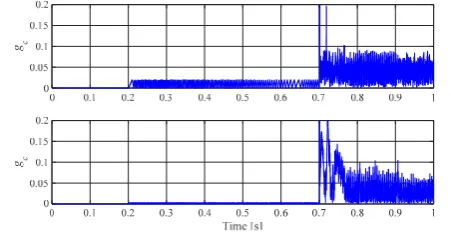
[image:5.595.318.547.406.529.2] [image:5.595.54.274.553.673.2] [image:5.595.318.545.560.683.2]

states corresponding to the minimum value of cost function gc for the two MPC strategies. The results are shown only for operation under load (i.e. t > 0.9s). The cost functions for the two MPC implementations are compared in Fig. 14 for the entire acquisition period. It can be observed that the M2_{PC does}

[image:6.595.50.276.158.279.2]

have a worse cost function performance at the instant when the speed step is applied (in line with flux control deterioration of Fig. 8); however, the cost function minimization performance is superior to FCS-MPC everywhere outside this time interval.

Fig. 14.Cost function minimization performance of the two MPC implementations for direct flux and current vector control. Top: FCS-MPC, bottom: M2_PC.

VI. CONCLUSION

Model predictive control for direct flux and current vector control of an induction machine is presented. The two MPC strategies, namely FCS-MPC and M2_{PC, are implemented and}

the performance is compared with the linear (PI) controller based approaches. While the FCS-MPC demonstrates greater robustness in the flux loop, it does produce greater harmonic content in the stator current. The M2_{PC strategy closely}

matches the performance of PI regulators while at the same time affording the benefits of MPC. By limiting the voltage command for the flux regulation, the machine’s total phase current can be limited to safe values; this feature is not available for FCS-MPC due to its inherent modulator-less nature.

The idea is initially introduced for simple speed-controlled drives but will be extended to torque control mode for experimental work to evaluate dynamic performance for torque control required for many applications such as traction. Flux loop performance with MTPA operation can be evaluated to give a comparison with PI-based implementation. The modulated MPC strategy will also be adopted for the direct flux and current vector control of permanent magnet synchronous machines in a future work.

VII.APPENDIX

The IM nameplate data and parameters are: rated voltage 400V, rated current 5.08A, frequency 50 Hz, rated speed 1400 rpm, rated torque 15 Nm, Rs=3.37 Ω (25°C), Rr=2.2 Ω (25°C), Lls=Llr=16 mH, Lm-unsat. = 283.3 mH.

References

[1] J. A. Rossiter, Model-Based Predictive Control: A Practical Approach, CRC Press, 2005.

[2] D. Bao-Cang, Modern Predictive Control, CRC Press, 2010.

[3] E. F. Camacho, C. Bordons, Model Predictive Control, London: Springer, 1998.

[4] L. Grune, J. Pannek, Nonlinear Model Predictive Control: Theory and Algorithms, Springer: Communications and Control Engineering Series, 2010.

[5] IET Control Engineering Series, Nonlinear Predictive Control: theory and practice, Edited by: B. Kouvaritakis, M. Cannon, Somerset, 2001. [6] S. Vazquez, J. I. Leon, L. G. Franquelo, J. Rodriguez, H A. Young, A.

Marquez, P. Zanchetta, “Model Predictive Control – A Review of Its Applications in Power Electronics”, IEEE Industrial Electronics Magazine, vol. 8, no. 1, pp. 16-31, March 2014.

[7] P. Karamanakos, T. Geyer, N. Oikonomou, F. D. Kieferndorf, S. Manias, “Direct Model Predictive Control – A Review of Strategies That Achieve Long Prediction Intervals for Power Electronics”, IEEE Industrial Electronics Magazine, vol. 8, no. 1, pp. 32-43, March 2014. [8] P. Cortés, M. P. Kazmierkowski, R. M. Kennel, D. E. Quevedo, J.

Rodríguez, “Predictive Control in Power Electronics and Drives”, IEEE Trans. on Ind. Elect., vol. 55, no. 12, pp. 4312-4324, December 2008. [9] P. Correa, M. Pacas, and J. Rodríguez, “Predictive Torque Control for

Inverter-Fed Induction Machines”, IEEE Trans. on Ind. Elect., vol. 54, no. 2, pp. 1073-1079, April 2007.

[10] Y. Zhang, H. Yang, “Model Predictive Torque Control of Induction Motor Drives With Optimal Duty Cycle Control”, IEEE Trans. on Power Elect., vol. 29, no. 12, pp. 6593-6603, December 2014.

[11] Y. Zhang, H. Yang, “Model-Predictive Flux Control of Induction Motor Drives With Switching Instant Optimization”, IEEE Trans. on Energy Conv., vol. 30, no. 3, pp. 1113-1122, September 2015.

[12] H. Guzman, M. J. Duran, F. Barrero, L. Zarri, B. Bogado, I. G.Prieto, M. R. Arahal, “Comparative Study of Predictive and Resonant Controllers in Fault-Tolerant Five-Phase Induction Motor Drives”, IEEE Trans. on Ind. Elect., vol. 63, no. 1, pp. 606-617, January 2016.

[13] F. Wang, S. Li, X. Mei, W. Xie, J. Rodríguez, R. M. Kennel, “Model-Based Predictive Direct Control Strategies for Electrical Drives: An Experimental Evaluation of PTC and PCC Methods”, IEEE Trans. on Ind. Inform., vol. 11, no. 3, pp. 671-681, June 2015.

[14] M. Habibullah, D. D. Lu, “A Speed-Sensorless FS-PTC of Induction Motors Using Extended Kalman Filters”, IEEE Trans. on Ind. Elect., vol. 62, no. 11, pp. 6765-6778, November 2015.

[15] E. Fuentes, D. Kalise, J. Rodríguez, R. M. Kennel, “Cascade-Free Predictive Speed Control for Electrical Drives”, IEEE Trans. on Ind. Elect., vol. 61, no. 5, pp. 2176-2184, May 2014.

[16] F. Wang, Z. Chen, P. Stolze, J. Stumper, J. Rodríguez, and R. M. Kennel, “Encoderless Finite-State Predictive Torque Control for Induction Machine With a Compensated MRAS”, IEEE Trans. on Ind. Inform., vol. 10, no. 2, pp. 1097-1106, May 2014.

[17] P. Alkorta, O. Barambones, J. A. Cortajarena, A. Zubizarrreta, “Efficient Multivariable Generalized Predictive Control for Sensorless Induction Motor Drives”, IEEE Trans. on Ind. Elect., vol. 61, no. 9, pp. 5126-5134, September 2014.

[18] C. A. Rojas, J. Rodríguez, F. Villarroel, J. R. Espinoza, C. A. Silva, M. Trincado, “Predictive Torque and Flux Control Without Weighting Factors”, IEEE Trans. on Ind. Elect., vol. 60, no. 2, pp. 681-590, Febraury 2013.

[19] L. Tarisciotti, P. Zanchetta, A. Watson, J. C. Clare, M. Degano, S. Bifaretti, “Modulated Model Predictive Control for a Three-Phase Active Rectifier”, IEEE Trans. on Ind. Appl., vol. 51, no. 2, pp. 1610-1620, March/April 2015.

[20] G. Pellegrino, R. I. Bojoi, and P. Guglielmi, “Unified Direct-Flux Vector Control for AC Motor Drives,” IEEE Trans. on Ind. Appl., vol. 47, no. 5, pp. 2093–2102, October 2011.

[21] G. Pellegrino, E. Armando, P. Guglielmi, “Direct Flux Field-Oriented Control of IPM Drives With Variable DC Link in the Field-Weakening Region”, IEEE Trans. on Ind. Appl., vol. 45, no. 5, pp. 1619–1627, November/December 2015.

[22] S. A. Odhano, R. Bojoi, A. Boglietti, S. G. Rosu, G. Griva, “Maximum Efficiency per Torque Direct Flux Vector Control of Induction Motor Drives”, IEEE Trans. on Ind. Appl., vol. 51, no. 6, pp. 4415–4424, November/December 2015.

[23] S. A. Odhano, “Self-Commissioning of AC Motor Drives,” Doctoral thesis, Department of Energy, Politecnico di Torino, Italy, 2014. [24] P. Cortes, J. Rodriguez, C. Silva, A. Flores “Delay Compensation in

Model Predictive Current Control of a Three-Phase Inverter”, Letters in IEEE Trans. on Ind. Elect., vol. 59, no. 2, February 2012.