University of Warwick institutional repository: http://go.warwick.ac.uk/wrap
This paper is made available online in accordance with
publisher policies. Please scroll down to view the document
itself. Please refer to the repository record for this item and our
policy information available from the repository home page for
further information.
To see the final version of this paper please visit the publisher’s website.
Access to the published version may require a subscription.
Author(s): Xuejuan Zhang, Gongqiang You, Tianping Chen and
Jianfeng Feng
Article Title: Maximum Likelihood Decoding of Neuronal Inputs from an
Interspike Interval Distribution
Year of publication: 2009
Link to published version:
http://dx.doi.org/10.1162/neco.2009.06-08-807
Maximum Likelihood Decoding of Neuronal Inputs
from an Interspike Interval Distribution
Xuejuan Zhang
Mathematical Department, Zhejiang Normal University, Jinhua, 321004, and Mathematical Department, Shaoxing University, Shaoxing, 312000, P.R.C.
Gongqiang You
Mathematical Department, Shaoxing University, Shaoxing, 312004, P.R.C.
Tianping Chen
Centre for Computational Systems Biology, Fudan University, Shanghai, 312000, P.R.C.
Jianfeng Feng
Centre for Computational Systems Biology, Fudan University, Shanghai, 312000, P.R.C., and Department of Computer Science, Warwick University,
Coventry CV4 7AL, U.K.
An expression for the probability distribution of the interspike interval of a leaky integrate-and-fire (LIF) model neuron is rigorously derived, based on recent theoretical developments in the theory of stochastic pro-cesses. This enables us to find for the first time a way of developing maximum likelihood estimates (MLE) of the input information (e.g., af-ferent rate and variance) for an LIF neuron from a set of recorded spike trains. Dynamic inputs to pools of LIF neurons both with and without interactions are efficiently and reliably decoded by applying the MLE, even within time windows as short as 25 msec.
1 Introduction
Neurons receive and emit spike trains, which are typically stochastic in nature due to the combination of their intrinsic channel fluctuations, the failure of their synaptic vesicle releases, and the variability in the input they receive. As a consequence, how to accurately and efficiently read out the input information from spike waves (simultaneously recorded multispike trains) remains elusive and is one of the central questions in (theoretical)
neuroscience (Rieke, Warland, & Steveninck, 1997; Gerstner & Kistler, 2002; Feng, 2003; Memmesheimer & Timme, 2006; Cateau & Reyes, 2006). For a given neuron or neuronal network, the most commonly used method to read out the input information is undoubtedly the maximum likelihood estimate (MLE), which is optimal under mild conditions. However, in or-der to rigorously perform the MLE, the prerequisite is knowing the exact expression of the interspike interval (ISI) distribution of efferent spikes of a neuron or a neuronal network. This is a difficult task in general. Even for the simplest leaky integrate-and-fire (LIF) model with constant input, such a distribution, which is equivalent to the first-passage of an Ornstein-Uhlenbeck (OU) process, was only obtained from the numerical inversion of its Laplace transform (Gerstner & Kistler, 2002; Tuckwell, 1988).
Other than in neuroscience, the first passage time of an OU process is also of prominent importance in many other fields, such as physics, engineering, and finance, and the topic has been widely addressed in many textbooks (Stratonovich, 1967; Risken & Frank, 1984; Gardiner, 1985). Thanks to recent developments (G ¨oing-Jaeschke & Yor, 2003; Alili, Patie, & Pedersen, 2005) in stochastic process theory, three expressions of the interspike interval distribution have become available. The first two are deterministic methods based on the knowledge of Laplace transform of the first hitting time, and the third is a probability method in which the probability density of ISIs can be numerically simulated by the Monte Carlo method. Here we prefer to implement the third one, based on which the maximum likelihood estimate (MLE) for the LIF model is successfully developed. Despite the fact that the MLE for a spiking neural model has been discussed intensively by a few authors (Deneve, Latham, & Pouget, 1999; Sanger, 2003; Feng & Ding, 2004; Paninski, Pillow, & Simoncelli, 2004; Ditlevsen & Lansky, 2005; Truccolo & Eden, 2005), to the best of our knowledge, our approach is the first one based on the exact expression of the ISI distribution of the LIF model.
MLE is employed. Therefore, the stochasticity in spikes does not contradict the time constraint.
Certainly neurons in a microcolumn interact with each other. By includ-ing lateral inhibition and the time delay of the synaptic inputs, we find that the input information can still be reliably read out from spike waves of an interacting neuronal network using the MLE strategy mentioned above. The results should open up many new and challenging problems for further research in both theory and application. For example, we would ask how to implement MLE for multilayer interacting spiking neuronal networks.
2 Theoretical Results
2.1 Probability Distribution of ISIs of an LIF Neuron. We start our discussion from a single LIF model. When the membrane potentialV(t) is below the thresholdVth, its dynamics is determined by
d V= −V
γdt+d Isyn(t),V≤Vth, (2.1)
withV(0)=Vrest<Vthand whereγis the decay time constant. The synaptic input is
Isyn(t)=a m
i=1 Ei−b
n
j=1 Ij,
where Ei = {Ei(t),t≥0}, Ij = {Ij(t),t≥0} are inhomogeneous Poisson processes with ratesλE,iandλI,j, respectively (Shadlen & Newsome, 1994),
a>0,b>0 are the magnitudes of each excitatory postsynaptic potential (EPSP) and inhibitory postsynaptic potential (IPSP), andmandnare the total number of active excitatory and inhibitory synapses. OnceV(t) crosses
Vthfrom below, a spike is generated, andVis reset toVrest, the rest potential. If there are numerous presynaptic inputs, we can use diffusion approxi-mation to approximate the synaptic inputs (Tuckwell, 1988). For simplicity, we further assumeVrest=0,a =b,m=n. Thus, the LIF model is simplified as
d V= −V
γdt+μdt+ √
σd Bt,V≤Vth (2.2)
with
μ=aλ(t)(1−r)
where λ(t)=iλE,i(t) andrλ(t)=
jλI,j(t), r is the ratio between the inhibitory input and the excitatory input. Ifμ(t)γ =Vth, the input is termed
exactly balanced inputbecause it ensures that the stable state ofV(t) is Vth, provided that noise is absent. Actually, the exactly balanced condition is equivalent to the following balanced relationship betweenλandr:
r(t)=1− Vth
aλ(t)γ. (2.4)
Biologically, equation 2.4 roughly describes the well-known push-pull effect of the inhibitory input to maintain the balanced inputs: the stronger the input (largerλ) is, the stronger the inhibitory input (largerr) is.
Feng and Ding (2004) derived an MLE formula of the input rateλunder the exactly balanced condition, equation 2.4. However, finding the exact MLE of the input for the general case remains an open question. In this letter, we develop an MLE strategy without this restriction, and both the input rateλand the ratior(or equivalently,σ) can be decoded at the same time. The idea of developing an MLE strategy of decoding both the input rate and the ratio between the inhibitory input and the excitatory input is interesting for biological applications (see section 4). One could easily adopt our approach to estimate other sets of parameters.
Let us first consider static inputs. The ISI of the efferent spikes can be expressed as
T=inf{t>0 :V(t)≥Vth|V(0)=0}, (2.5)
which is a random variable. More precisely, we should define
τi =inf{t> τi−1:V(t)≥Vth|V(τi−1)=0},i≥1,
τ0=0, (2.6)
andTi =τi−τi−1,i≥1. It is readily seen that{Ti,i≥1}is an independent and identically distributed (i.i.d.) sequence and has the identical probability density asT.
By setting U=(V−μγ)/√σ, the distribution of the ISIs of efferent spikes of the LIF model, equation 2.2, is equivalent to the distribution of the first-passage time of the following OU process,
dU= −U
starting atUre = −√μγσ to hitUth= Vth√−σμγ. The corresponding ISIs of efferent spikes can be expressed as
T=inf{t>0 :U(t)≥(Vth−μγ)/
√
σ|U(0)= −μγ /√σ}. (2.8)
Letpλ,r(t) be the probability density ofT. As mentioned above, the first-passage time problem, which occurs in many areas, was once believed to have no general explicit analytical formula (Gerstner & Kistler, 2002), except a momentary expansion of the first-passage time distribution for constant input. Recently Alili et al. (2005) summarized what we know about the density of the first-passage time of an OU process, where three expressions of the distribution ofT—the series representation, the integral representa-tion, and the Bessel bridge representation—are presented. For numerical approximation, the authors pointed out that the first two approaches are easy to implement but require knowledge of the Laplace transform of the first hitting time, which can be computed only for some specific continuous Markov processes, while the Bessel bridge approach overcomes the prob-lem of detecting the time at which the approximated process crosses the boundary (Alili et al., 2005). For this reason, we prefer to apply the Bessel bridge method under which the probability density ofThas the following form (see the appendix),
pλ,r(t)=exp
−V2
th+2μγVth
2γ σ +
t
2γ
p(0)(t)
×E0→Vth
exp
− 1
2γ2σ
t
0
(vs−Vth+μγ)2ds
, (2.9)
where
p(0)(t)= Vth
√
2πσt3exp
−Vth2 2tσ
(2.10)
is the probability density of the nonleaky integrate-and-fire model and
{vs}0≤s≤tis the so-called three-dimensional Bessel bridge from 0 toVthover the interval [0,t]. Mathematically, it satisfies the following stochastic differ-ential equation:
dvs=
Vth−vs
t−s + σ vs
ds+√σd Bs, 0<s<t, v0=0, vt =Vth. (2.11)
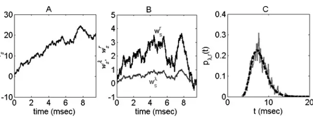
Figure 1: (A). Sampling trajectory of{vs}0≤s≤tfrom 0 toVth=20. (B). Sampling trajectories of {wsλ}0≤s≤t,{wrs}0≤s≤t, which are the derivatives of{vs}0≤s≤t with respect toλandr, respectively. (C).pλ,r(t) (dashed curve) and histogram (solid curve) from a direct simulation of the LIF model.
At first glance, the expression of probability density 2.9 looks some-what complicated, as it is an expectation of a singular stochastic process. However, we can use the Monte Carlo method to numerically evaluate the expectation. To do this, we have to generate a large number, sayM, of inde-pendent sampling paths of a three-dimensional Bessel bridge. It should be pointed out that in numerical simulations, we do not use equation 2.11 to directly simulate the process{vs}0≤s≤tsince it is degenerate ats=0. Instead we consider the process{v2
s}0≤s≤t, which satisfies
d(vs)2=2vsdvs+σds. (2.12)
Note that the second term on the right-hand side of the equation above is due to the Ito integral. According to this, the iterating procedure to simulate the stochastic processvsis as follows (we simply denotev(j) asv(jt)):
⎧ ⎪ ⎪ ⎪ ⎪ ⎪ ⎨ ⎪ ⎪ ⎪ ⎪ ⎪ ⎩
u(j+1)=u(j)+t·
2v(j)(Vth−v(j))
t−jt +3σ
+2v(j)·√σ·B(j),
v(j+1)=u(j+1),
with v(1)=0,u(1)=0 and where tis the time step. B(j)= B(jt+ t)−B(jt) is the increment of the Brownian motion with distribution
Norm (0, t). The three-dimensional Bessel bridgevs has a trajectory as shown in Figure 1A.
Denote{vi(kt)}theith sampling trajectory, and let
f1(t)=exp
−V2
th+2μγVth
2γ σ +
t
2γ
[image:7.432.65.371.69.185.2]
Then the approximation formula for equation 2.9 is
¯
pλ,r(t)= f1(t)· 1 M
M
i=1 exp
− 1
2γ2σ
n
k=1
(vi(kt)−Vth+μγ)2·t
,
(2.13)
wheret= t
n. The ISI density calculated frompλ,r(t) is plotted in Figure 1C, which demonstrates that ¯pλ,rmatches the histogram obtained from a direct simulation of the LIF model very well.
2.2 MLE Decoding Strategy. Having an exact function of the distribu-tion pλ,r(t), we can perform the MLE decoding procedure. The likelihood function is given by
L(λ,r)= N
i=1
pλ,r(Ti), (2.14)
whereNis the total number of spikes. Then
lnL(λ,r)= N
i=1
lnpλ,r(Ti). (2.15)
The optimal estimate of the input information (λ,r) corresponds to the root of the equation,
⎧ ⎪ ⎪ ⎨ ⎪ ⎪ ⎩
∂lnL(λ,r)
∂λ =0
∂lnL(λ,r)
∂r =0
. (2.16)
Denotewx s
=dvs/dx(x=λ,r). As the density functionpλ,r(t) includes a singular stochastic process{vs}0≤s≤t whose derivatives with respect toλ andr, that is,{wsλ}0≤s≤tand{wrs}0≤s≤t, are also singular stochastic processes, we should pay additional attention to calculate∂lnL/∂x (x=λ,r). First, let us derive the equation ofwx
s(x=λ,r). It follows from equation 2.11 that
wx
s (x=λ,r) satisfies the following equation,
dws=
−wx s
t−s + σ
x
vs −
σ v2 s wx s
ds+ σ
x
2√σd Bs, x=λ,r, (2.17)
whereσx= ∂σ∂x,v0=0 andwx0=0 (x=λ,r). Sampling trajectories ofwsλ andwr
Let
f2(t)=exp
− 1
2γ2σ
t
0
(vs−Vth+μγ)2ds
;
then
lnpλ,r(t)=lnf1(t)+lnE0→Vth[f2(t)].
The derivatives of f1(t) and f2(t) are
∂
∂xlnf1(t)=hx+ V2
thσx 2σ2t,
with
hx= V
2
thσx 2σ2γ +
(μxσ−μσx)Vth
2σ2 −
σ
x 2σ,
and
gx(t)= ∂
∂xf2(t)
= f2(t)· σ
x 2σ2γ2
t
0
(vs−Vth+μγ)2−2σ
σ
x
(vs−Vth+μγ)
·(wxs +μxγ)
ds, x=λ,r. (2.18)
Then
∂
∂xlnE0→Vth[f2(t)]=
E0→Vth
∂
∂xf2(t)
E0→Vth[f2(t)]
= E0→Vth[gx(t)]
E0→Vth[f2(t)] .
Therefore,
∂lnL
∂x =N·hx+ V2
thσx 2σ2
N
i=1
Ti−1+ σ
x 2σ2γ2
N
i=1
E0→Vth[gx(Ti)]
E0→Vth[f2(Ti)]
, x=λ,r.
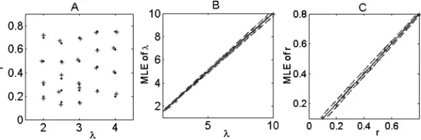
Figure 2: MLE of a single neuron. (A). MLE of (λ,r) from 1000 interspike intervals. Dots represent true values, while stars are estimated from the MLE method. (B). MLE (star points) ofλ versus the input rateλ for a fixed ratio
r =0.25. (C). MLE (star points) ofrversus the input raterfor a fixed input rate λ=7. Parameters areVth=20 mV,γ =20 msec, anda=2.
Substituting equation 2.16 with 2.19, we know that the MLE of the input information (λ,r) is the root to the following two equations:
N·hλ+V
2
thσλ
2σ2
N
i=1 Ti−1+
σ λ
2σ2γ2
N
i=1
E0→Vth[gλ(Ti)]
E0→Vth[f2(Ti)]
=0, (2.20)
N·hr+ V
2
thσr 2σ2
N
i=1 Ti−1+
σ
r 2σ2γ2
N
i=1
E0→Vth[gr(Ti)]
E0→Vth[f2(Ti)]
=0. (2.21)
Though it is difficult to find an analytical solution to equations 2.20 and 2.21, we can numerically find its root, denoting it as ( ˆλ, ˆr). Figure 2A depicts the value ( ˆλ, ˆr) versus its actual value (λ.r) for the model defined by equation 2.2, where each point of ( ˆλ, ˆr) is obtained by using 1000 interspike intervals. It is clearly shown that the estimated value ( ˆλ, ˆr) almost exactly matches the true value (λ.r).
Let us look at the Fisher information in our model. Define
I1(λ,r)=
⎡ ⎢ ⎢ ⎢ ⎣ E
∂lnpλ,r(t)
∂λ
2 E
∂lnpλ,r(t)
∂λ
∂lnpλ,r(t)
∂r
E
∂lnpλ,r(t)
∂λ
∂lnpλ,r(t)
∂r
E
∂lnpλ,r(t)
∂r 2 ⎤ ⎥ ⎥ ⎥ ⎦. (2.22) As
∂lnpλ,r(t)
∂x =hx+ V2
thσx 2σ2t +
σ
x 2σ2γ2
E0→Vth[gx(t)]
E0→Vth[f2(t)]
, x=λ,r,
we can numerically calculate the four terms in the above matrix—for example,
I1(λ,r)11=
hλ+ V
2
thσλ
2σ2t +
E0→Vth[gλ(t)]
E0→Vth[f2(t)]
2
pλ,r(t)dt,
I1(λ,r)12=
hλ+ V
2
thσλ
2σ2t + σ
λ
2σ2γ2
E0→Vth[gλ(t)]
E0→Vth[f2(t)]
×
hr+V
2
thσr 2σ2t +
σ
r 2σ2γ2
E0→Vth[gr(t)]
E0→Vth[f2(t)]
pλ,r(t)dt.
We also calculate the other two elements. The Fisher information matrix is defined as
I(λ,r)=NI1(λ,r).
For a given sampling numberN, we have
( ˆλ,rˆ)→Norm((λ,r),I(λ,r)−1),
in the distribution sense, or briefly,
( ˆλ,rˆ)≈Norm((λ,r),I(λ,r)−1).
The confidence intervals of the model parameters ( ˆλ,rˆ) for a givenNcan be computed as
λ−(I(λ,r)−1) 11, λ+
(I(λ,r)−1) 11 , r−
(I(λ,r)−1) 22,r+
(I(λ,r)−1) 22
where (I(λ,r)−1)
ii is theiith component of the inverse Fisher information matrix.
In Figures 2B and 2C, we plot the confidence intervals for parametersλ andr for N=1000, respectively. Interestingly, one can see that the confi-dence interval of the parameterλis enlarged, while the confidence interval of the ratio parameterr becomes smaller with the increase of input fre-quency. As Feng and Ding (2004), pointed out, the higher the input rate, the more variable the output spikes (i.e., the larger the CV, the smaller the Fisher information). This is why we observe such opposite increasing properties of the confidence intervals by noticing that increasing the ratio between the in-hibitory input and the excitatory input tends to decrease the CV of the firing.
Remark. In our toy model here, we assume that the input takes the form of a Poisson process. Hence, the remaining variable in the input variance could be the ratioror the EPSP magnitude. It is easily seen that our approach is equivalent to estimating the input mean and variance, although we estimate λ,rhere. Certainly in many cases, the ratioris fixed in a biological circuit. Suppose that only the input rateλis to be decoded. The MLE ofλis the root to equation 2.20. The corresponding Fisher information is then given by
I(λ)=E
∂lnpλ(t)
∂λ
2 =
hλ+V
2
thσλ
2σ2t +
E0→Vth[gλ(t)]
E0→Vth[f2(t)]
2
pλ(t)dt,
(2.23)
wherepλ(t) has the same expression as equation 2.9 but withrbeing fixed.
Thus, to estimate the single parameterλ, the confidence interval is
λ− 1
NI(λ), λ+ 1
NI(λ)
. (2.24)
2.4 Comparison with Rate Decoding. One might ask why we do not decode the input information by simply fitting the firing rate and CV since the first and second moments of ISIs are known. Such a rate decoding approach has been extensively discussed in the literature. It is known that when the sampling number is large enough, both MLE and rate coding methods give reasonable results. However, from the viewpoint of parameter estimation, the advantage of the MLE method is obvious. By the Cram´er-Rao lower bound, we know that MLE is optimal but rate decoding is not.
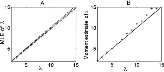
Figure 3: Comparison of two methods. (A) Estimate of afferent inputλvia the MLE method. Dashed lines are confidence intervals calculated from equation 2.24. (B). Estimate of afferent inputλvia the rate coding method. Here we fix
r=0,a=1 and choose 200 ISI intervals.
the decoding error using the MLE method is bounded by the Cram´er-Rao lower bound, while the error using the rate coding approach may be out of this range. From this point of view, the MLE is optimal. The advantage of the MLE over rate coding is quite obvious even for a relatively small sampling number (here we takeN=200).
3 MLE of Dynamic Inputs
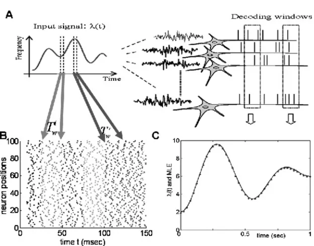
3.1 Decoding of Dynamic Inputs in Networks Without Interactions. Usually a postsynaptic neuron receives dynamic inputs from presynaptic neurons, and we have to decode the input within a short time window. Based on the above decoding strategy, let us now further employ the MLE to decode dynamic inputs in pools of neurons. The network is composed of 100 neurons, as schematically plotted in Figure 4A. We assume that the input is varying slowly compared with the timescale of the neuronal dy-namics, so that in each time window of fixed lengthTW, the ISI distribution adiabatically follows the stationary one.
Under the exactly balanced condition, equation 2.4, the problem has been investigated by Rossoni and Feng (2007). However, the method presented there cannot be extended to a more general case without knowing the exact relationship between the input and the output of the LIF neuron. Nevertheless, on the basis of this theoretical development, we can now relax the restriction of the exactly balanced condition and read out both the input rate and variance from spike waves in a short time window (see Figure 4B).
Figure 4: MLE in a network without interactions. (A) Schematic plot of reading dynamic inputs from an ensemble of neurons. For a fixed time window (indi-cated byTi
w,Twj), the spikes are collected and the input is decoded by means of MLE. (B) Raster plot of spikes in five different decoding windows. The infor-mation is read out from the spikes in each window. (C) An example of reading out the dynamic input rates from an ensemble of neurons. The original signal λ(t) is plotted in the continuous line, while dots are estimated values ofλ(t).
other ratios between the inhibitory input and the excitatory input. We sup-pose that the waveform of input isλ(t)=2+4(sin2(2πt)+sin2(3
2πt)). Here the timescale of the input is measured in seconds; thus, it varies slowly compared with the timescale of the neuronal dynamics. Note that during the decoding procedure, any ISI longer thanTwwill not be included in the
MLE estimate, so the estimated input ˆλ(t) is bound to be biased—a typical situation in survival analysis. To obtain an unbiased estimate, the censored intervals have to be included, and more detailed calculations are required. However, the numerical results (see Figure 4C) indicate that the bias is very limited, and we simply ignore the issue of censored intervals here.
Figure 4C depicts the MLE versus the input frequency for time windows
Tw =25 ms. Although Tw is very short, we can see that the estimate is
excellent (except that it is slightly downward biased).
sensory inputs and motor outputs is around 200 msec. They then argued that only a few interspike intervals could be used to estimate the input in each layer, and therefore a stochastic dynamics is implausible in the nervous system. Our results clearly show that within a very short time window (∼25 msec), the spikes generated from an array of neurons contain enough information for the central nervous system to decode the input information. Hence, even without the overlap of the processing time of each layer in the nervous system, within 200 msec it could reliably read out the information for around 10 layers.
3.2 Decoding of Input Information in Networks with Interactions. So far we have assumed that neurons in the same column are regraded as independent. Certainly neurons in a microcolumn interact with each other, which might considerably change all conclusions in the previous sections. Can we or the central nervous system read out the input information from spike waves? In this section, we further investigate such an issue. The purpose is to read out the information of an external stimulus even in the presence of interactions between neurons in a microcolumn.
The strategy adopted here (or possibly by the nervous system) is based on including the lateral inhibition and the time delay of the synaptic inputs. As a result, all neurons in a network behave independently before the inter-actions kick in. The depolarization caused by the external inputs evokes the hyperpolarizing effect of inhibitory interactions between neurons, which subsequently shuts down the firing of all neurons (first epoch) and enables the neurons in the microcolumn to act independently again.
The model we consider here consists of PE =100 excitatory and PI = 100 inhibitory neurons with all-to-all connectivity. The corresponding LIF equation for each neuron is
d Vj
dt = − Vj
γ +IjE(t)+ISj(t), Vj ≤Vth, j=1,2, . . . ,Nn=PE+PI, (3.1)
where
⎧ ⎪ ⎪ ⎪ ⎨ ⎪ ⎪ ⎪ ⎩
IjE(t)=aλj(t)+a
λj(t)ξj(t),
IjS(t)= PE
k=1
tm k+τ<t
wE
jkδ(t−tkm−τ)−rE I PI
l=1
tm l+τ<t
wI
jlδ(t−tlm−τ).
(3.2)
In the equation,IE
j(t) is the external input from the stimulus with an input rateλj(t) and magnitudea,ξj(t), and j =1, . . . ,Nnare independent white noises. IS
j(t) is the spiking input from other neurons to the jth neuron.
wE
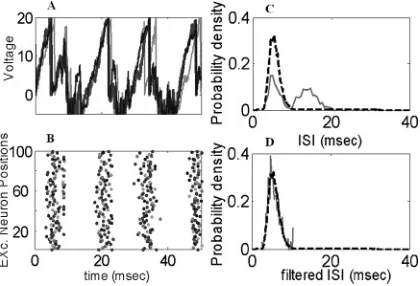
Figure 5: (A) Trajectories of three excitatory neurons in an interacting network forλ=4,D=2. (B) Raster plots of 100 excitatory neurons. (C) The histogram (solid curve) obtained from a direct simulation of the model and the theoretical density (dashed curve). (D) The solid curve is the histogram from the filtered interspike intervals (the first modes inC); the dashed one is the same as inB.
jthneuron receives from thekth and thelth neurons,rE Iis the ratio between the inhibitory and the excitatory interactions,tm
k is themth spike generated from thekth neuron, andτ is the synaptic time delay. We suppose that wE
jk andwIjl are uniformly distributed in [0,D] (Dis termed the maximal coupling strength or, simply, the coupling strength), andλi(t)=λj(t)=λ(t). In our numerical simulations, we fixa=1,τ=5 msec,rE I =1.8.
Figures 5A and 5B show one simulation with the setup as above by fixing
D=2. As expected, with the application of the external inputs, all neurons start responding, and some fire a few spikes. However, once the inhibitory neurons fire, they send spikes to other neurons, which causes a hyperpolar-ization effect on these postsynaptic neurons, and all neuronal activities are shut down after a certain time delay of the synaptic transmission. Once the network becomes silent, the interactions between neurons disappear, and neurons in the network act as independent units again. Hence the external inputs evoke the second epoch of the spikes. This procedure repeats itself. Consequently, the network will produce rhythmic oscillations by properly cooperating the local inhibition and the time delay of the synaptic transmis-sion, a well-known phenomenon observed in many biological experiments. In noisy networks of LIF neurons, it is shown that the oscillation frequency is of the order of the inverse of the synaptic delay (Brunel & Hakim, 2008). Here we will investigate how the network rhythm is related to information decoding.
[image:16.432.111.321.75.218.2]that the former exchange information continuously, while the latter only react to each other when the membrane potential exceeds a threshold that results in the independent phases in Figure 5B.
Based on such an inhibition-induced shutting-down mechanism, let us now investigate how afferent input rateλ(t) can be read out accurately by applying the MLE strategy. The problem of introducing interactions in a fixed time window is that the decoding may have a significant bias. To resolve this issue, we first look at the histogram of the ISIs of equation 2.3 in the case that the input rateλ(t) is time independent, say,λ(t)=λ=4. It is clearly indicated in Figure 5C that the histogram now has two modes: the one with short ISIs corresponds to the actual ISIs driven by the external input, and the other is due to the interactions. After filtering out the second mode, the obtained histogram fits well with the theoretical density (the dashed trace in Figure 5D). To decode the input information, we filter out the spikes corresponding to the second mode and exclusively use the ISIs of the first mode. We will show that in a short time window, the input rate can be reliably decoded.
In Figures 6A and B, we test our algorithm in a dynamic input with waveform λ(t)=2+4(sin2(2πt)+sin2(3
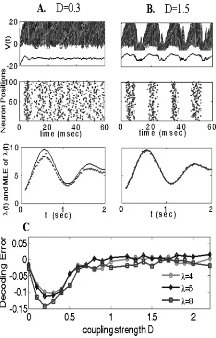
2πt)), for different values of cou-pling strength. Heretis measured in seconds, which ensures the ISI distri-bution being adiabatically stationary in each time window of length around 25 msec. To show the network behaviors under different coupling intensi-ties, the ensemble voltage traces and the corresponding raster plots of 100 excitatory cells for λ(t)=λ=3 are depicted in the top and middle pan-els of Figures 6A and 6B, respectively. Interestingly, the network displays rhythmic activity when the coupling strength is strong and the decoding (shown in the bottom trace of Figure 6B) is quite accurate; however, for weak values of the coupling strength, no rhythmic activities are observed, and, as expected, the estimated values (see the bottom trace of Figure 6A) are much less accurate than in the rhythmic case.
Figures 6A and 6B suggest that there should exist a critical value of the coupling strengthDc, after which the network can perform decoding accurately. To see this, we plot the relative decoding error λˆ−λλ versus the coupling intensity Din Figure 6C, for constant afferent inputs (we choose λ=4, λ=5, andλ=8). ForD=0, the decoding is very accurate, which is the case discussed in section 3.1. When Dslightly increases, the absolute decoding error increases. This is because the interactions between neurons cannot be shut down for weak coupling strengths. After about D=0.25, the absolute decoding error gradually decreases, and after about D=0.8, the input rate can be reliably read out; meanwhile, the network exhibits clear rhythmic activities.
Figure 6: MLE in a network with interactions. (A, B) Top traces: The trajecto-ries of 100 excitatory neurons and the corresponding mean voltages forλ=3 during 0∼60 ms. Middle traces: Raster plots corresponding to the above trace. Bottom traces: Reading out the dynamic inputs (the solid curve) from 100 ex-citatory neurons, every dot is estimated by the MLE approach within a fixed time window ofTw=25 msec. Left column is forD=0.3, and right column is for D=1.5. (C) The optimal coupling intensities for reading out the input information within a fixed time windowTw=25 msec.
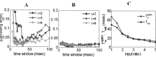
Figure 7: (A) Decoding errors of reading out intermediate input rates within different time windows, where optimal time windows are shown to be around 15 to 40 msec. (B) Decoding errors of reading out high input rates are shown to be very small within both short and large time windows. (C) Relationship of the optimal decoding windows and the periods of the network oscillations. For moderate input rates,Toptim
w ≈Tnet.D=1.5.
optimal windows exist and are around 15 to 40 msec, which are in the gamma range; for a high input rateλ, the decoding errors are small (<5%) for both the short and long time windows. The accuracy of decoding with high input rates stems from the fact that spikes are generated within a very short time (5 msec or less, the synaptic delay time), which implies that neurons in a pool have no time to interact with each other before starting the next epoch of firings. Hence, in response to a high input rate, neurons in a network act independently. This is why a small decoding error is achieved even for long time windows.
To explore how the optimal decoding windows for moderate input rates come about and how they are related with the periodsTnetof the network oscillations, we further depict these two time windows (Tnet and Twoptim)
versus the input rate λ in Figure 7C. The definition of Tnet is clear (see Figure 6B). For a reasonable range of input ratesλ(about 2≤λ≤5), the optimal decoding windows are approximately equal to the network peri-ods. The consistency of the optimal decoding windows and the periods of the network oscillations for moderate input rates shows that the spikes generated from a pool of neurons within the period of the network rhythm are sufficient to read out input rates. Time windows that are too small or too large will either have insufficient input information or redundant inter-spike intervals, both of which will introduce bias in decoding. The results in Figures 6 and 7 may serve as a good example to show the functional role of the gamma rhythm (30 to 80 Hz) in information processing, which has been extensively discussed by many authors (see Buzs´aki, 2006).
[image:19.432.64.371.72.185.2]neurons, say 1000 LIF neurons, are grouped intoN=10 columns, and each 100 neurons in a same column share an identical tuning curve defined by
λ(xi;x(t))=λ0+c·λ0exp
−(x(t)−xi)2 2d2
, (3.3)
wherecis a constant scaling factor,dis the tuning width,xiis the column’s field center, andxis the position. For example, the neuron in theith column receives an input that is the position information x(t)∈[0,L] (we take
L=11 here), and the response of the neuron is given byλ(xi,x(t)). The task is to read out the position informationx(t). The setup mimics the situation of reading out the position of a rat from simultaneous recordings of place cells in hippocampus (Truccolo & Eden, 2005).
For simulation, we fixc=2,d=1.5, and λ0=2. We assume that the target positionxchanges in time according tox(t)=Nj=1ξjχ(t∈Ij), where
ξj are independent random variables uniformly distributed in [0,L], and
Ij = {t: (j−1)Tw<t< j Tw}, that is, we consider a target hopping everyTw
to a new random position between 0 and L. An outcome of our performance is shown in Figure 8.
Let us further investigate the tracking problem within interacting neu-ronal networks. The setup is similar to that in Figure 8A. An ensemble of 2000 LIF neurons is grouped into 10 columns. Neurons in different columns do not have interaction, but each 200 neurons in the same column interact with each other in an all-to-all connection with equations 3.1 and 3.2, and these 200 neurons share an identical tuning curve defined by equation 3.3. Figure 9A depicts the tuning curve and the estimate ofλ(x;xi) by using the MLE method described above. The task of the tracking problem is to read out the position informationx(t). As shown in Figure 9B, the decoding is still accurate even though neurons in the network interact with each other.
4 Discussion
Figure 8: MLE in position tracking (the network is without interactions). (A) Setup of encoding and decoding. The place informationx(t) is fed to 1000 neurons organized in 10 columns with different preferred positionxi. For each column, spikes are collected in the windowTw, and the MLE is applied. The position is read out by first solving equation 3.3, obtaining the corresponding
ˆ
x, and fitting a gaussian curve to all 10 data points ˆx. The maximum point of the fitted gaussian curve is the decoded position. (B) One example of ˆλversus columns. (C) An example of 10 decoded results of stimulus positions.
[image:21.432.83.349.441.544.2]rhythm in signal decoding) elsewhere. Furthermore, our approach may help us to answer another long-standing problem: What is the ratio between inhibitory and excitatory inputs in a biological neuron? Although it has been found that the number of inhibitory neurons is smaller than the number of excitatory neurons in the cortex (Shadlen & Newsome, 1998; Leng et al., 2001), it is generally agreed that inhibitory neurons send stronger signals than excitatory neurons (Destexhe & Contreras, 2006). Therefore, the exact ratio between inhibitory and excitatory inputs remains elusive. With the MLE developed in this letter, we may be able to reliably estimate the ratio between inhibitory and excitatory inputs to a LIF neuron.
As a simplified phenomenological neuronal model, the LIF equation preserves spiking properties of a neuron, and the input information can be reliably read out, as we show here. However, the LIF model fails to capture many biophysical details. Some other models are more biophysi-cally accurate but still mathematibiophysi-cally simple, such as quadratic IF neurons (Feng & Brown, 2000a; Brunel & Latham, 2003), exponential IF neurons (Fourcaud-Trocme, Hansel, van Vreeswijk, & Brunel, 2003), and, more re-cently, adaptive exponential IF neurons (Brette & Gerstner, 2005). It is shown that adaptive exponential IF neurons give an effective description of neuron activities and can reliably predict the voltage trace of a naturalistic pyra-midal neuron from a dynamic I-V curve (Badel et al., 2008). We realized that generalizing the MLE strategy developed for the LIF neurons to these nonlinear IF neurons needs more investigation, as it is not easy to derive exact expressions of the distributions of ISIs for these nonlinear IF neurons.
Appendix: Derivation of Equation 2.9
The probability density of the first hitting time of an Ornstein-Uhlenbeck (OU) process has been presented in the literature (G ¨oing-Jaeschke & Yor, 2003; Alili et al., 2005). However, readers who are not familiar with stochas-tic process theory may not follow the mathemastochas-tical proof there. In this appendix, we provide a derivation of equation 2.9 and explain the proba-bility meaning of the expression.
A.1 Some Preliminary Results. We first introduce some stochastic pro-cesses related to equation 2.9.
LetB= {B t}t≥0be a Brownian motion starting at B0=xwith its incre-mentBt+t−Bt∼N(0, t). Ifx=0, thenBis called a standard Brownian motion. DenotePB M
x the corresponding probability law defined on the fol-lowing sampling space,
where{Xt}t≥0 is the canonical process, withFt=σ{Xs,s≤t}being infor-mation before timet.
The OU process starting fromx∈Rwith parameterα∈Ris the solution to the following stochastic differential equation:
dUt =d Bt−αUtdt, U0=x∈R. (A.1)
Under the canonical measure PB M
x , this process is no longer a Brownian motion. We hope to find a new law, denoted asPxOU(α), under which the pro-cessWt = Bt−
t
0Usds,t≥0 is still a Brownian motion. Using the Girsanov theorem (the same idea was also employed in Feng & Brown (2000b)), we find that such a new law exists, and the density transformation from PB M
x toPxOU(α)along the canonical path is given by
d PxOU(α)
d PB M x
(ω)=exp
−α
2(B 2
t −x2−t)−
α2 2
t
0 Bs2ds
. (A.2)
Based on the Brownian motion, we can have another stochastic process, the so-called three-dimensional Bessel process{R(t)}t≥0starting atR0=0, which is constructed from three independent standard Brownian motions
{Bi,t}t≥0,i=1,2,3:
Rt=
B2
1,t+B22,t+B32,t,t≥0. (A.3)
Rt is actually the unique solution to the following stochastic differential equation,
d Rt=d Bt+n−1
2Rt dt, R0=x≥0, (A.4)
withn=3, based on the following two facts:
1. The increment of a Brownian motion is of the order√dt, thusd B2
t = 2Btd Bt+dt.
2. For two independent standard Brownian motions,
B1,td B1,t+B2,td B2,t=
B2
1,t+B22,td Bt,
whereBtis another standard Brownian motion.
A Brownian bridge {Bsx,y}0≤s≤t from x to y of length t is a Brownian motion, given (B0=x,Bt=y). Mathematically, it can be expressed as
Bsx,y=x+Bs+s
Starting from three independent Brownian bridge{Bi0,,s0}0≤s≤t,i =1,2,3, the process
Rxs,y
= x+s
t(y−x)+B 0,0 1,s
2 +!B20,,s0
"2 +!B30,,s0
"2
,0≤s≤t (A.6)
is the three-dimensional Bessel bridge fromxtoyof lengtht. Similar to the derivation of equation A.4 from A.3,{Rxs,y}0≤s≤tcan be characterized as the solution to the following stochastic process:
drs=
1
rs +
y−rs
t−s
ds+d Bs, 0<s<t, r0=x,rt=y. (A.7)
A.2 Distribution of the First Passage Time of the OU Process. Let
{Xt}t≥0be a stochastic process and
τa =inf{t≥0 :Xt =a},
that is,τa is the first hitting time of the process{Xt}t≥0ata. Under the law PB M
x , it is known that
PB M
x (τa ∈dt)=
a−x √
2πt3exp
−(a−x)2
2t
dt, f or a≥x. (A.8)
Our purpose is to seek the distribution ofτaunder lawPxOU(α). According to equation A.2, we know that
d POU(α)
x (τa ∈dt)
= {τa∈dt}
exp
−α
2(a
2−x2−t)−α2 2
t
0 Bs2ds
d PxB M
=exp
−α
2(a
2−x2−t)
·ExB M
exp
−α2
2 t
0 Bs2ds)
I{τa∈dt}
=exp
−α
2(a
2−x2−t)
·ExB M
exp
−α2
2 t
0 Bs2ds
## ##τa =t
·PB M
x (τa ∈dt), (A.9)
whereEB M
A Brownian motion starting atx, givenτa =t, is a Brownian bridge from
xtoaof lengtht, givenτa =t. We write such a conditional Brownian bridge as
!
Bsx,a,0≤s≤τa|τa =t "
. (A.10)
LetYx,a
s =a+x−Btx−,as,0≤s≤t, also a bridge fromxtoa of lengtht. Since a Brownian bridge is gaussian, it is known that
!
Bsx,a,0≤s≤t " d
=!Ysx,a,0≤s≤t "
(A.11)
by checking the first and the second moments; here· · ·= · · ·d means “equal in a distribution sense.”
Furthermore, givenτa =t, it is easily seen that
σa =sup{s:Ysx,a =a,0≤s≤t} =sup{s:B x,a
τa−s =x,0≤s≤τa} =τa. (A.12)
This implies that iftis the first hitting time of the bridge{Bx,a
s }0≤s≤t ata, thentis the last visiting time of the bridge{Yx,a
s }0≤s≤tata. Equations A.11 and A.12 tell us that we can replace the Brownian bridge (Bx,a
s ,0≤s≤t), givenτa =t, by a new bridge (Ysx,a,0≤s≤t) without conditions.
Then what is the law for this new bridge? Thanks to the Williams time-reversal theorem, the process (Yx,a
s ,0≤s≤t) has the same distribution as a three-dimensional Bessel bridgeRx,a
s fromxtoaof lengtht, which is the solution to equation A.7. As a rigorous proof for this result requires deep mathematical techniques related to stochastic processes, we will not repeat here but refer readers to corollary 4.4 in Revuz and Yor (1999).
We can now calculateEB M
x [·|τa =t]. First, from an important fact that the process (Bx,a
s ,0≤s≤t) under the law PxB Mis identical to (a−Bsx,a,s≥0) under the lawPB M
a−x, we conclude that fora ≥x,
EB M x
exp
−α2
2 t
0 B2
sds ##
##τa =t
=EB M a−x
exp
−α2
2 t
0 (
a−Bs)2ds ##
##τ0=t
. (A.13)
Second, based on the fact we discussed above that (Ba−x,0
s ,0≤s≤
lengtht, we have
EaB M−x
exp
−α2
2 t
0
(a−Bs)2ds ##
##τ0=t
=EaBes−x
exp
−α2
2 t
0
(Rs−a)2ds ##
##Rt=0
. (A.14)
Third, based on
E0Bes[f(Rs)|Rt =a−x]=E[f(Rs)|R0=a−x,Rt =0]
=E[f(Rt−s)|R0=0,Rt=a−x],
we know that
EaBes−x
exp
−α2
2 t
0
(Rs−a)2ds ##
##Rt=0
=E0Bes
exp
−α2
2 t
0
(Rt−s−a)2ds ##
##Rt=a−x
=E0Bes
exp
−α2
2 t
0
(Rs−a)2ds ##
##Rt =a−x
=E0→a−x
exp
−α2
2 t
0
(rs−a)2ds
, (A.15)
where E0→a−x[·] stands for the expectation of three-dimensional Bessel bridge{rs}s≤t from 0 toa−xover the interval [0,t], which is the solution to equation A.7.
Therefore,
d POU(α)
x (τa ∈dt)=exp
−α
2(a
2−x2−t)
·E0→a−x
exp
−α2
2 t
0
(rs−a)2ds
·PxB M(τa ∈dt),
(A.16)
SetPxOU(α)(τx∈dt)= p(xα→)a(t)dt, and together with equation A.8, we have
p(xα→)a(t)=exp
−α
2(a
2−x2−t)
p(0)0→a−x(t)
·E0→a−x
exp
−α2
2 t
0
(rs−a)2ds
By replacingx= −√μγσ,a = Vth√−μγ
σ ,α=γ1 and lettingvs =√σrs, we ob-tain the density equation 2.9 of ISIs of an LIF model, equation 2.2, and the corresponding three-dimensional Bessel bridge{vs}0≤s≤t from 0 toVth, which satisfies equation 2.11.
Acknowledgments
We are grateful to the referees for their useful comments, which im-proved this letter greatly. We benefited from discussions with M. P. Qian, E. Rossoni, and J. S. Xie. J.F. was partially supported by the CARMEN e-science project (www.carmen.org.uk) funded by the EPSRC (EP/ E002331/1) and an EU grant BION. X.J. was partially supported by the National Natural Science Foundation of China (under grant nos. 10305007, 10771155) and a Foundation for the Author of National Excellent Doctoral Dissertation of PR China.
References
Alili, L., Patie, P., & Pedersen, J. L. (2005). Representations of the first hitting time density of an Ornstein-Uhlenbeck process.Stochastic Models,21, 967–980. Badel, L., Lefort, S., Brette, R., Petersen, C. C. H., Gerstner, W., & Richardson, M. J. E.
(2008). Dynamic I-V curves are reliable predictors of naturalistic pyramidal-neuron voltage traces.J. Neurophysiol.,99(2), 656–666.
Brunel, N., & Hakim, V. (2008). Sparsely synchronized neuronal oscillations.Chaos,
18, 015113.
Brunel, N., & Latham, P. E. (2003). Firing rate of the noisy quadratic integrate-and-fire neuron.Neural Computation,15, 2281–2306.
Brette, R., & Gerstner, W. (2005). Adaptive exponential integrate-and-fire model as an effective description of neuronal activity.J. Neurophysiol.,94, 3637–3642. Buzs´aki. G. (2006).Rhythms of the brain. New York: Oxford University Presss. Cateau, H., & Reyes, A. D. (2006). Relation between single neuron and population
spiking statistics and effects on network activity.Phys. Rev. Lett.,96, 058101. Deneve, S., Latham, P. E., & Pouget, A. (1999). Reading population codes: A neural
implementation of ideal observers.Nat. Neurosci.,2, 740–745.
Destexhe. A., & Contreras, D. (2006). Neuronal computations with stochastic net-work states.Science,314, 85–90.
Ditlevsen, S., & Lansky, P. (2005). Estimation of the input parameters in the Ornstein-Uhlenbeck neuronal model.Phys. Rev. E,71, 011907.
Feng, J. F. (Ed.). (2003).Computational neuroscience: A comprehensive approach. London/ Boca Raton, FL: Chapman and Hall/CRC, Press.
Feng, J. F., & Brown, D. (2000a). Integrate-and-fire models with nonlinear leakage.
Bull. Math. Biol.,62(3), 467–481.
Feng, J., & Brown, D. (2000b). Impact of correlated inputs on the output of the integrate-and-fire models.Neural Computation,12, 671–692.
Fourcaud-Trocme, N., Hansel, D., van Vreeswijk, C., & Brunel, N. (2003). How spike generation mechanisms determine the neuronal response to fluctuating inputs.
J. Neurosci.,23, 11628–11640.
Gardiner, C. W. (1985).Handbook of stochastic methods: For physics, chemistry and the natural sciences. Berlin: Springer.
Gerstner, W., & Kistler. W. (2002).Spiking neuron models single neurons, populations, plasticity. Cambridge: Cambridge University Press.
G ¨oing-Jaeschke, A., & Yor, M. (2003). A clarification note about hitting times densities for Ornstein-Uhlenbeck processes.Finance Stoch.,7, 413–415.
Hung, C. P., Kreiman, G., Poggio, T., & DiCarlo, J. J. (2005). Fast readout of object identity from macaque inferior temporal.Science,310, 863–866.
Leng, G., Brown, C. H., Bull, P. M., Brown, D., Scullion, S., Currie, J., et al. (2001). Responses of magnocellular neurons to osmotic stimulation involves coactivation of excitatory and inhibitory input: An experimental and theoretical analysis.J. Neurosci.,21, 6967–6977.
Memmesheimer, R. M., & Timme, M. (2006). Designing the dynamics of spiking neural networks.Phys. Rev. Lett.,97, 188101.
Paninski, L., Pillow, J. W., & Simoncelli, E. P. (2004). Maximum likelihood estimation of a stochastic integrate-and-fire neural encoding model.Neural Computation,16, 2533–2561.
Revuz, D., & Yor, M. (1999).Continuous martingales and Brownian motion(3rd ed.). Berlin: Springer.
Rieke, F., Warland, D., & Steveninck, R. (1997).Spikes: Exploring the neural code. Cambridge, MA: MIT Press.
Risken, H., & Frank, T. (1984).The Fokker-Planck equation: Methods of solutions and applications. Berlin: Springer-Verlag.
Rossoni, E., & Feng, J. F. (2007). Decoding spike ensembles: Tracking a moving stimulus.Biol. Cybern.,96, 99–112.
Sanger, T. D. (2003). Neural population codes.Curr. Opin. Neurobiol.,13, 238–249. Shadlen, M. N., & Newsome, W. T. (1994). Noise, neural codes and cortical
organi-zation.Curr. Opin. Neurobiol.,4(4), 569–579.
Shadlen, M. N., & Newsome, W. T. (1998). The variable discharge of cortical neurons: Implications for connectivity, computation, and information coding.J. Neurosci.,
18, 3870–3896.
Stratonovich, R. L. (Ed.). (1967).Topics in the theory of random noise: Mathematics and its applications. Gordon and Breach Science Pub.
Truccolo, W., & Eden, U. (2005). A point process framework for relating neural spik-ing activity to spikspik-ing history, neural ensemble and covariate effects.J. Neurophys.,
93, 1074–1089.
Thorpe, S., Fiz, D., & Marlot, C. (1996). Speed of processing in the human visual system.Nature,381, 520–522.
Tuckwell, H. C. (1988). Introduction to theoretical neurobiology. Cambridge: Cambridge University Press.