Return on Universal Education: SSA Case Study on Bihar

Munich Personal RePEc Archive

Return on Universal Education: SSA

Case Study on Bihar

Dinda, Soumyananda

Department of Economics, The University of Burdwan, Department

of Economics, Sidho-Kanho-Birsha University

25 January 2015

Return on Universal Education: SSA Case Study on Bihar

Soumyananda Dinda

Department of Economics, University of Burdwan, West Bengal, India

Email: [email protected]

Abstract

Mass universal education is a necessary condition for initiation of economic development in

underdeveloped and backward state like Bihar in India. The Govt. of India has taken initiative for

universal mass education and prime focus is on Sarbha Shikhsha Abhijan (SSA). This study attempts

to assess the impact of universal education programme such as SSA in Bihar. The difference –in-

difference (DD) approach is used here to measure the impact of SSA treatment on unorganised sector

in Bihar. This study finds that literate people earn Rs. 43 higher than that of illiterate, and SSA is

giving additional return nearly more than Rs. 600 Crore per annum only from small and tiny

enterprise in urban Bihar.

Key Words: DD, Difference –in-Difference, Control group, Treatment, SSA, Universal Mass Education, Bihar, income, Return on Education, unorganised sector, development.

1. Introduction

Education is the cornerstone of economic growth and social development. Schooling is

desirable for individual as well as for society. At macro level, a better-educated workforce

enhances a nation’s stock of human capital that is crucial for raising productivity and

economic development (Barro, 1996; Romer, 1986; Lucas, 1988; Ravallion and Chen, 1997).

One of the crucial problems of economic development is the problem of accounting for

income pattern and related other social issues; one of them is the educational externality

(Lucas 1988). There are different opinions regarding the presence of external effect of human

capital. However, it is difficult to capture the externality of human capital. In Lucas (1988),

human capital is found to have positive external effect on aggregate production function. In

the presence of external effect, the social and private return to human capital differs. There

exists a substantial empirical literature relating human capital accumulation to economic

growth. In 50s and 60s Gary Becker, Jacob Mincer, T.W. Schultz and other economists focus

on the role of education on economic development. Recently, Lucas (1988), Barro (1991),

education externalities improve literature on it. The positive externalities associated with

human capital are given importance in the new growth theories, and in most of these dynamic

models externality result in the returns to scale in the production sector. Basic question here

is: How do we measure the educational externalities? Applying difference in difference (DD)

approach, this paper attempts to assess the impact of education, especially measuring the

returns of education.

Truly, acquiring education is an investment in the sense that one gives up something now in

the hope of getting more back in future. For that reason, education is often described as

‘human capital’, the title of a famous book by Gary Becker. So, spending on education should

be considered as the investment. Like all investments, how the future gain compares to the

current sacrifice is critical in determining whether education is a good investment or not.

What is the factor motivating individual to determine for acquiring education. The basic

assumptions are (i) earning of individual depends on year of schooling; i.e., one individual

has s year of (post compulsory) schooling, earning is W(s). (ii) Assume there is no direct cost

but cost of education is only forgone earnings. (iii) Assume everyone lives forever. So,

present discount value (PDV) of s years of education is:

Taking log of both sides of the above equation can be written as

First order condition can be written as

Acquiring education up to the point where the increase in log earnings is equal to the rate at

which future earnings are discounted.

Suppose all individuals are identical and require different levels of education in equilibrium,

then must be the case that

is equalised for different levels of s. The coefficient on s is the measure of r– rate of return to

education1.

Economics scholars have invested much energy in identifying the value of educational

investment, to determine whether governments and individuals are investing optimally. Much

of this work stems from the work of Becker (1962) that introduced the concept of treating

investment in education as a capital investment. Since then research scholars mainly focus on

1_{From empirical findings it is clear that typical OLS estimates from an earnings function are about 2.2} – _12.8

percent which suggests that education is a good investment.

 

rt rS

s

PDV e W s dt W s e

r

  









 

 

log

PDV



log

W S

 

rS

log

r





 

 

log PDV logW S  rS log r

 

 

W s

r

estimation of the return to education investment2. However, estimates of the return vary

significantly, depending on the data sets used, the assumptions made and the estimation

techniques.

Furthermore, attempts at estimating a single rate of return may not be very informative if

returns to education differ by education level, or differ across populations (including by

social strata). This may be particularly important for policy responses, but ironically gets

masked by methodological debates. Similarly, economists often fail to take into account the

risk associated with education investment decisions. Risk may play an important role in an

individual’s education investment decision, and indeed a government’s educational

investment level, and should be taken into consideration when testing rationality and

optimality of education investment (see Heckman, Lochner, and Todd 2008) and the

comprehensive review in Heckman et al. (2006)). In addition, as most cogently argued by

Oreopoulos and Salvanes (2011), the return to education may be much wider than the private

financial returns that is the focus of so much of the economics literature, and perhaps

economics as a profession has allowed a major body of research on the non-pecuniary returns

(which may create private returns through externalities that are as great – if not greater – than

the direct effect of education on earnings) to become dominated by the other social sciences.

Education is the key treatment that may remove major hindrance of social development and

economic growth. Educated workforce enhances a nation’s stock of human capital which

increases productivity and economic development (Barro 1996; Romer 1986; Lucas 1988;

Ravallion and Chen 1997). Education is associated with high rates of return, both private and

social. So, schooling is desirable for all. There is an increasing focus on achieving universal

primary education in developing countries like India. In this context, primary education has

the highest social rates of return in developing countries (Psacharooulos and Patrinos 2004).

Is it true in India? How far is it true in backward state like Bihar also? This study attempts to

answer this question focusing on universal primary education in Bihar.

The government of India has launched the Sarbha Shikha Avijan (SSA) to improve the

literacy level and endeavours to achieve universal primary education since 1987-88. Across

states this SSA programme is more or less successful. In this context, especially this paper

focuses on Bihar, which is one of the least developed states in India. Recently a high rate of

2

growth is observed and consequently speedy development starts to gain momentum in Bihar.

Basic question what is the reason behind it. There are several reasons but one of them is the

improvement of education level in Bihar. Has any impact of education on Bihar economy? In

other word, what is the return of education in Bihar? How do we measure it?

This study attempts to answer the above questions especially in the context of Bihar. This

paper is organised as follows: Section 2 explains the methodological issues. Section 3

describes data. Section 4 analyses results, and finally concludes.

2. Methodology: Difference in Difference Approach

Recently the most popular identification strategy in applied work is the difference in

difference (DD) methodology (see Dinda 2015 for details). Application of DD is a very

simple random assignment with treatment and comparison. One group is treated with

intervention and other is control group. DD is the application of two-way fixed effects model

having cross sectional and time series data. So, basically we have pre and post data for group

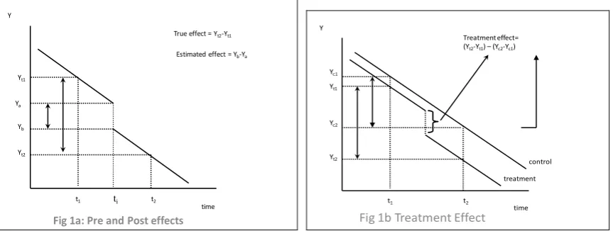
receiving intervention. Suppose treatment intervention occurs at ti and we observe outcome

Yt1 at t1 and post treatment outcome Yt2 at t2. Fig 1 (Fig 1a & Fig 1b) show the treatment

effect. Using time series data, true effect is the difference between pre and post observed

outcome, i.e., (Yt2–Yt1) but actual estimated effect of the treatment is (Yb–Ya).

Fig 1a: Pre and Post effects

time Y

t1 t2

Ya

Yb

Yt1

Yt2

True effect = Yt2-Yt1

Estimated effect = Yb-Ya

ti

Fig 1b Treatment Effect

time Y

t1 t2 Yt1

Yt2

treatment control Yc1

Yc2

Treatment effect= (Yt2-Yt1) –(Yc2-Yc1)

We use time series of untreated group to establish what would have occurred in the absence

of the intervention. Here, the key concept is the control (c) and treatment (t). Table 1 display

Table 1: Difference in Difference approach

Difference in Difference

Before After

Difference Group 1

(Treat)

Yt1 Yt2 ΔYt

= Yt2-Yt1

Group 2 (Control)

Yc1 Yc2 ΔYc

=Yc2-Yc1

Difference ΔΔY

ΔYt– ΔYc

Control group identifies the time path of outcomes that would have happened in the absence

of the treatment. In this example, Y changes by (Yc2 – Yc1) even without the intervention.

Treatment group identifies the time path of outcomes that would have happened in the

intervention of the treatment. In this case, Y changes by (Yt2 – Yt1) with the intervention.

Here, impact measurement is the difference in the change in outcomes, i.e., (Yt2–Yt1) –(Yc2–Yc1),

or, treatment effect is ( ∆∆Y = ) ∆Yt - ∆Yc .

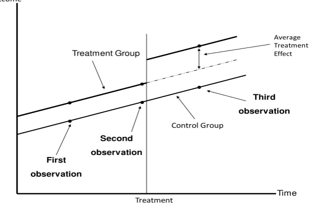
Fundamental assumption that trends (slopes) are same in treatments and controls. It is true for sometimes. Truly we need minimum three time point observations as depicting in fig 2.

Time

Treatment Outcome

Treatment Group

Control Group

Average Treatment Effect

First

observation

Second

observation

Third

observation

Fig 2: Pre and Post Observations

Following Dinda (2015), We evaluate the impact of treatment or program on an outcome Y over population individuals.

Model

Suppose there are two groups indexed by treatment status T = 0, 1; where 0 and 1 indicate

individuals who do not receive treatment (i.e., the control group) and individuals who receive

treatment (i.e., treatment group), respectively. Assume that we observe individuals in two

time periods, t = 0, 1 where 0 indicates a time period before the treatment group receives

treatment (i.e. pre-treatment), and 1 indicates a time period after the treatment group receives

individuals will typically have two observations each, one pre-treatment and one

post-treatment. For the sake of notation let 𝑌̅̅̅̅₀𝑇 and 𝑌̅̅̅̅₁𝑇 be the sample averages of the outcome for

the treatment group before and after treatment, respectively, and let 𝑌̅̅̅̅₀𝐶 and 𝑌̅̅̅̅₁𝐶 be the

corresponding sample averages of the outcome for the control group. Subscripts correspond

to time period and superscripts to the treatment status.

2.2 Modelling the Outcome

The outcome Yi is modelled by the following equation

𝑌𝑖 = 𝛽0+ 𝛽1 𝑇𝑖+ 𝛽2 𝑡𝑖+ 𝛽3 (𝑇𝑖∗ 𝑡𝑖) + 𝜀𝑖 (1)

where the 𝛽₀, 𝛽₁, 𝛽₂, 𝛽₃, coefficients are all unknown parameters and εi is a random,

unobserved "error" term which contains all determinants of Yi which the model omits. By

inspecting the equation we should observe the coefficients and have the following

interpretation

𝛽0 = constant term, 𝛽1 = treatment group specific effect (to account for average permanent

differences between treatment and control), 𝛽₂ = time trend common to control and treatment

groups, 𝛽₃ = true effect of treatment

The purpose of the program evaluation is to find a “good” estimate of δ, 𝛿̂, given the data that

we have available.

2.3 Assumptions for an Unbiased Estimator

A reasonable criterion for a good estimator is that it be unbiased which means that "on

average" the estimate will be correct, or mathematically that the expected value of the

estimator

𝐸[𝛽̂] = 𝛽3 3

The assumptions we need for the difference in difference estimator to be correct are given by

the following

1) The model in equation (Outcome) is correctly specified. For example, the additive

structure imposed is correct.

2) The error term is on average zero: E [εi] = 0. Not a hard assumption with the constant

term 𝛽₀ put in.

3) The error term is uncorrelated with the other variables in the equation:

Cov (εi, Ti) = 0

Cov (εi, ti) = 0

the last of these assumptions, also known as the parallel-trend assumption, is the most

critical.

Under these assumptions we can use equation (Outcome) to determine that expected values

of the average outcomes are given by

𝐸[𝑌₀𝑇] = 𝛽₀+ 𝛽₁

𝐸[𝑌₁𝑇] = 𝛽₀+ 𝛽₁+ 𝛽₂+ 𝛽₃

𝐸[𝑌₀𝐶] = 𝛽₀

𝐸[𝑌₁𝐶] = 𝛽₀+ 𝛽₂

These equations are helpful to identify the estimated impact of a treatment.

2 The Difference in Difference Estimator

Before explaining the difference in difference estimator it is best to review the two simple

difference estimators and understand what can go wrong with these. Understanding what is

wrong about as an estimator is as important as understanding what is right about it.

2.1 Simple Pre versus Post Estimator

Consider first an estimator based on comparing the average difference in outcome Yi before

and after treatment in the treatment group alone3.

𝛿̂ = 𝑌̅1 1𝑇− 𝑌̅0𝑇 (D1) Taking the expectation of this estimator we get

𝐸[𝛿̂ ] = 𝐸[𝑌̅_{1 1}𝑇] − 𝐸[𝑌̅₀𝑇]

= [𝛽₀+ 𝛽₁+ 𝛽₂+ 𝛽₃] – [𝛽₀+ 𝛽₁]

= 𝛽₂+ 𝛽₃

which means that this estimator will be biased so long as 𝛽₂ ≠ 0, i.e. if a time-trend exists in

the outcome Yi then we will confound the time trend as being part of the treatment effect.

2.2 Simple Treatment versus Control Estimator

Next consider the estimator based on comparing the average difference in outcome Yi

post-treatment, between the treatment and control groups, ignoring pre-treatment outcomes4_.

𝛿2

̂ = 𝑌̅1𝑇− 𝑌̅1𝐶 (D2) Taking the expectation of this estimator we get

𝐸[𝛿̂ ] = 𝐸[𝑌̅_{2 1}𝑇] − 𝐸[𝑌̅₁𝐶]

= [𝛽₀+ 𝛽₁+ 𝛽₂+ 𝛽₃] – [𝛽₀+ 𝛽₂]

3

This would be the estimate one would get from an OLS estimate on a regression equation of the form on the sample from the treatment group only.

4

= 𝛽₁+ 𝛽₃

So, this estimator is biased so long as 𝛽₁ ≠ 0, i.e. there exist permanent average differences

in outcome Yi between the treatment groups. The true treatment effect will be confounded by

permanent differences in treatment and control groups that existed prior to any treatment.

Note that in a randomized experiments, where subjects are randomly selected into treatment

and control groups, β1 should be zero as both groups should be nearly identical: in this case

this estimator may perform well in a controlled experimental setting typically unavailable in

most program evaluation problems seen in economics.

2.3 The Difference in Difference Estimator

The difference in difference (or "double difference") estimator is defined as the difference in

average outcome in the treatment group before and after treatment minus the difference in

average outcome in the control group before and after treatment5 : it is literally a “difference

of differences”.

𝛿̂ = (𝑌̅𝐷𝐷 1𝑇− 𝑌̅0𝑇) − (𝑌̅1𝐶− 𝑌̅0𝐶) (DD) Taking the expectation of this estimator we will see that it is unbiased

𝐸[𝛿̂ ] = 𝐸[𝑌̅_{𝐷𝐷 1}𝑇] − 𝐸[𝑌̅₀𝑇] − (𝐸[𝑌̅₁𝐶] − 𝐸[𝑌̅₀𝐶])

=( [𝛽₀+ 𝛽₁+ 𝛽₂+ 𝛽₃] – [𝛽₀+ 𝛽₁]) – ([𝛽₀+ 𝛽₂]- 𝛽₀)

= [𝛽₂+ 𝛽₃] – (𝛽₂)

= 𝛽₃

This estimator can be seen as taking the difference between two pre-versus-post estimators

seen above in (D1), subtracting the control group’s estimator, which captures the time trend

𝛽2, from the treatment group’s estimator to get 𝛽3. We can also rearrange terms in equation

(DD) to get 𝛿̂ = (𝑌̅_{𝐷𝐷 1}𝑇− 𝑌̅₁𝐶) − (𝑌̅₀𝑇− 𝑌̅₀𝐶) in which it can be interpreted as taking the

difference of two estimators of the simple treatment versus control type seen in equation

(D2). The difference estimator for the pre-period is used to estimate the permanent difference

β1, which is then subtracted away from the post-period estimator to get 𝛽₃.

Now, in this context, simple econometrics model is Yit = β0 + β1Tit+ β2Ait + β3TitAit + εit ,

where Tit is individual treated and Ait is in the period when treatment occurs. TitAit is the

interaction term, treatment individual after the intervention.

5

T ab le 2 :

Yit = β0 + β1Tit + β2Ait + β3TitAit + εit

Before After

Difference

Group 1 (Treat)

β0+ β1 β0+ β1+ β2+ β3 ΔYt

= β2+ β3

Group 2 (Control)

β0 β0+ β2 ΔYc

= β2

Difference ΔΔY = β3

This DD methodology is used in several studies. Here, we also use the DD for a case study on

the return on education in Bihar. For this purpose we collect primary data from a field survey.

Data

We have collected data on unorganised sector focusing on the small and tinny enterprises

covering major urban Bihar during January – July, 2010. The small and tinny enterprises are

mostly self-employed (including street vendors) and do their own business as their livelihood.

They provide service to the municipal people and contribute to the urban economy. Total

number of business unit (population) in this specific unorganised sector in urban Bihar is

nearly than 3.5 lakhs. It mainly covers major municipal areas of towns and cities in Bihar.

Data are collected in different (three) rounds for cross checking and verifications. So, here,

we have a cross section data including thin and densely populated area. Using stratified

random sampling technique we have collected data taking several parameters. Finally, our

sample size is 2588. These data represent whole urban Bihar covering all districts towns

which are consist of words, roads, streets, lane and bye lanes etc.

Our main focus is to measure the impact of Sarbha Sikhsha Avijan (SSA) applying difference

in difference (DD) approach. Here, we consider that SSA is a treatment which has applied in

Bihar since early 1990s. We can apply DD methodology to assess the impact of SSA only

having control and treatment groups in pre and post SSA. In this context, we identify and set

up illiterate and literate as control and treatment groups, respectively. Individual has reported

their age in year. Now, using the ‘age’ variable we can identify individual weather he/she has

received the treatment of SSA or not, and hence we have pre and post SSA groups. SSA

starts in early 1990s in Bihar. Hence, individual did not receive SSA treatment if he /she was

born before 1988, otherwise, his/her age is more than 22 years and they belong to pre SSA;

(control) individual can be divided into sub-groups according to their age more than 22 years

or less such as pre and post control and pre and post treatment SSA. Thus, as per treatment

(SSA) and its availability during their childhood we formulate minimum 2x2 groups, i.e., pre

and post control as well as pre and post treatment groups in Bihar. Now, we investigate the

impact of SSA treatment in Bihar focusing different variables such as income, inequality, etc.

Results

Income of individual is considered here as outcome. For our purpose, we measure the return

of SSA treatment. There is a huge income difference between literate and illiterate. Fig 3

shows the monthly income difference between educated and illiterate.

Fig 3: Income difference

2800 2900 3000 3100 3200 3300 3400 Illiterate

Educated

Income (monthly)

Income also varies among literate people as per their education level. Fig 4 shows the

monthly income differences among educated people.

Fig 4: Income difference among educated people

3300 3400 3500 3600 3700 3800 3900 4000 4100 4200

Primary Upper Primary Secondary Higher edu

Primary results suggest that literacy drive (or education) has impact on income, but question

we examine alpha t- test for income of literate versus illiterate and the alpha t is 4.46 and

statistically significant. Table 4 displays pair wise alpha t-test and their significance levels.

Economic returns of secondary and higher education are higher than that of primary

education.

Table 4: Alpha t- test

Education Level Illiterate Primary Upper Primary Secondary

Educated 4.46***

Illiterate -

Primary 2.08**

Upper Primary 2.69*** 0.61

Secondary 7.46*** 3.71*** 2.3**

Higher Education 5.36*** 2.06** 1.17 -0.39

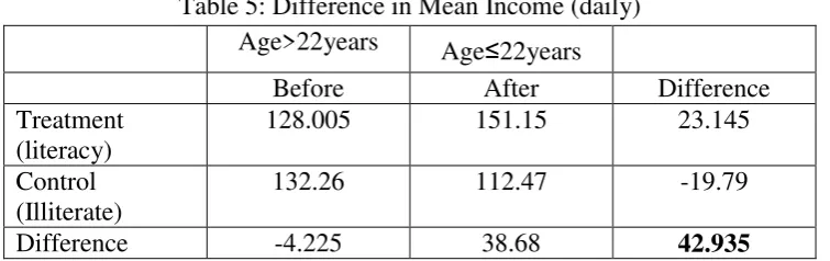
Table 5: Difference in Mean Income (daily)

Age>22years _{Age≤22years}

Before After Difference

Treatment (literacy)

128.005 151.15 23.145

Control (Illiterate)

132.26 112.47 -19.79

Difference -4.225 38.68 42.935

Table 5 presents the mean daily income differences using DD approach. Before SSA

treatment, average income of literate and illiterate are Rs. 128.0 and Rs. 132.26, respectively.

Post SSA treatment, average income of literate and illiterate are Rs. 151.15 and Rs. 112.47,

respectively. Mean daily income of literate is Rs. 38.68 more compare to illiterate in the post

SSA period. It suggests that on an average daily income of literate people earn Rs. 38.68

more compare to illiterate in the post SSA treatment period. Average daily income of literate

people rises by Rs. 23.15 due to SSA treatment. Applying DD approach, average daily

income of literate people is higher than that of illiterate due to SSA treatment. Literate people

earn on an average daily income of Rs. 42.93 or Rs 43 more than illiterate. Literate people

earn more annually Rs 12900 to Rs. 14200 compare to illiterate and estimated additional

annual income of Bihar is nearly Rs.645 Crore. Hence, literacy has positive impact on

income level of self employed people in the small and tiny enterprise sector in urban

economy of Bihar.

This paper attempts to assess the impact of mass universal education programme such as

Sarbha Shiksha Abhijan (SSA) in Bihar. Applying difference –in difference (DD) approach,

this paper attempts to measure the returns of SSA mass education in Bihar. SSA is giving

return more than Rs. 600 per annum only from small and tiny enterprise in urban Bihar. Now,

the govt. of Bihar realises the importance of universal primary education and has taken

initiative to improve education level, and automatically Bihar economy starts to growth with

overall development.

References:

Acemoglu, D. & Angrist, J.D. (2001). How Large are Human-Capital Externalities? Evidence

from Compulsory-Schooling Laws. In B. Bernanke & K. Rogoff, NBER Macroeconomics

Annual (9-59). Cambridge: National Bureau of Economic Research.

Ashenfelter, O. Harmon, C. & Oosterbeek, H. (1999). A Review of Estimates of the

Schooling/Earnings Relationship, with Tests for Publication Bias.” Labour Economics, 6 (3),

453–470.

Becker, G.S. (1962). Investment in Human Capital: A Theoretical Analysis. The Journal of

Political Economy, 70 (5), 9–49.

Card, D. (1999). The Causal Effect of Education on Earnings. In Ashenfelter, O. and Card,

D., Handbook of Labor Economics. Rotterdam: Elsevier.

Chevalier, A. (2011). Subject Choice and Earning of UK Graduates. Economics of Education

Review, Special Issue.

Dee, T.S. (2004). Are There Civic Returns to Education?.” Journal of Public Economics 88

(9-10), 1697–1720.

de la Fuente, A. & Ciccone, A. (2003). Human Capital in a Global and Knowledge-Based

Economy. European Commission: DG Employment and Social Affairs.

Devereux, P. & Fan, W. (2011). Earnings Returns to the British Education Expansion.

Economics of Education Review, Special Issue.

Dickson, Matt R. and Sarah Smith. 2011. “What Determines the Return to Education: An

Extra Year or a Hurdle Cleared?” Economics of Education Review, Special Issue.

Dinda, S. (2015). A Note on DD Approach. MPRA Paper 63949.

Green, F. & Zhu, Y. (2010). "Overqualification, Job Dissatisfaction, and Increasing

Harmon, C.P., Oosterbeek, H. & Walker, I. (2003). The Returns to Education:

Microeconomics. Journal of Economic Surveys, 17 (2), 115–155.

Harmon, C.P., Hogan, V. & Walker, I. (2003). Dispersion in the economic return to

schooling. Labour Economics, 10 (2), 205-214.

Haveman, R.H. & Wolfe. B.L. (1984). Schooling and Economic Well-Being: The Role of

Nonmarket Effects. Journal of Human Resources, 19 (3), 377–407.

Heckman, J.J., Lochner, L. & Todd, P. (2006). Earnings Functions, Rates of Return and

Treatment Effects: The Mincer Equation and Beyond. In E. Hanushek & F.Welch,

Handbook of the Economics of Education, 307–458, Rotterdam:Elsevier.

Harmon, C. (2011). Economic Returns to Education: What we know, what we don’t know,

and where we are going – some brief pointers. IZA Policy Paper No. 29.

Heckman, J.J., Lochner, L. & Todd P. (2008). Earnings Functions and Rates of Return.

Journal of Human Capital, 2 (1), 1–31.

Heckman, J.J., Tobias, J. & Vytlacil, E. (2001). Four parameters of interest in the evaluation

of social programs. Southern Economic Journal, 68 (2), 419-442.

Heckman, J.J. & Urzua, S. (2009). Comparing IV With Structural Models: What Simple IV

Can and Cannot Identify. National Bureau of Economic Research Working Paper 14706.

Heckman, J.J. & Vytlacil, E. (2005). Structural Equations, Treatment Effects and

Econometric Policy Evaluation. Econometrica, 73 (3), 669–738.

Henderson, Daniel J., Solomon J. Polachek and Le Wang. 2011. “Heterogeneity in Schooling

Rates of Return.” Economics of Education Review, Special Issue.

Lochner, Lance. 2004. “Education, Work, and Crime: A Human Capital Approach.”

International Economic Review 45 (3): 811–843.

Melnik, A., Pollatschek, M.A. & Comay, Y. (1973). The Option Value of Education and the

Optimal Path for Investment in Human Capital. International Economic Review, 14 (2), 421–

435.

Milligan, K., Moretti, E. & Oreopoulos, P. (2004). Does education improve citizenship?

Evidence from the United States and the United Kingdom. Journal of Public Economics, 88

(9), 1667–1695.

Oreopoulos, P. (2007). Do dropouts drop out too soon? Wealth, health and happiness from

compulsory schooling. Journal of Public Economics, 91 (11-12), 2213–2229.

Oreopoulos, P. & Salvanes, K.G. (2011). Priceless: The Nonpecuniary Benefits of Schooling.

Journal of Economic Perspectives, 25 (1), 159–84.

Returns. American Economic Review, 93 (3), 948–964.

Park, S. (2011). Returning to School for Higher Returns. Economics of Education Review,

Special Issue.

Walker, I. & Zhu, Y. (2008). The College Wage Premium and the Expansion of Higher

Education in the UK. Scandinavian Journal of Economics, 110 (4), 695-709.

Walker, I. & Zhu, Y. (2011). Differences by Degree: Evidence of the Net Financial Rates of

Return to Undergraduates. Economics of Education Review, Special Issue.

Psacharopoulos, G. and Patrinos, H. (2004). Returns to investment in education: A further