Abstract— In this paper, a new computational technique is presented based on the eXtended Finite Element Method for large deformation of metal forming processes. An ALE technique is employed to capture the advantages of both Lagrangian and Eulerian methods and alleviate the drawbacks of the mesh distortion in Lagrangian formulation. The X-FEM procedure is implemented to capture the discontinuities independently of element boundaries. The process is accomplished by performing a splitting operator to separate the material (Lagrangian) phase from convective (Eulerian) phase, and partitioning the Lagrangian and relocated meshes with some triangular sub-elements whose Gauss points are used for integration of the domain of elements. Finally, several numerical examples are presented to demonstrate the capability of enriched FE technique in large deformation of forming processes.
Index Terms— Metal forming, Extended FEM, ALE technique, Large deformation.
I. INTRODUCTION
In metal forming processes with large deformations, the note for mesh adaption in different stages of process is of great importance. The need for mesh conforming to the shape of the interface must be preserved at each stage of simulation. In numerical simulation, the requirement of mesh adaptation may consume high expenses of capacity and time. Thus, it is necessary to perform an innovative procedure to alleviate these difficulties by allowing the interfaces to be mesh-independent. In large deformation analysis with large mass fluxes, the conventional finite element technique using the updated Lagrangian formulation may suffer from serious numerical difficulties when the deformation of material is significantly large. This difficulty can be particularly observed in higher order elements when severe distortion of elements may lead to singularities in the isoparametric mapping of the elements, aborting the calculations or causing numerical errors [1]. In order to overcome this difficulty, the arbitrary Lagrangian– Eulerian (ALE) approach has been proposed in the literature [2, 3]. In ALE approach, the mesh motion is taken arbitrarily from
Manuscript received August 26, 2007.
This work was supported by the Iran National Science Foundation. Corresponding author. Tel. +98 (21) 6600 5818; Fax: +98 (21) 6601 4828; e-mail: [email protected] (Amir R. Khoei).
Center of Excellence in Structural and Earthquake Engineering, Department of Civil Engineering, Sharif University of Technology, P.O. Box. 11365-9313, Tehran, Iran.
material deformation to keep element shapes optimal. In ALE description, the choice of the material, spatial, or any arbitrary configuration yields to a Lagrangian, Eulerian, or arbitrary Lagrangian-Eulerian description, respectively.
The aim of present study is to develop the ALE technique in large deformation analysis using the X-FEM method based on an operator splitting technique. In the Lagrangian phase, a typical X-FEM analysis is first carried out with updated Lagrangian approach. The Eulerian phase is then applied to update the mesh, while the material interface is independent of the FE mesh. The main difficulty in ALE formulation of solid mechanics is the path dependent material behavior. The constitutive equation of ALE nonlinear mechanics contains a convective term which reflects the relative motion between the physical motion and the mesh motion.
II. THEEXTENDEDFINITEELEMENTMETHOD The enriched finite element method is a powerful and accurate approach to model discontinuities, which are independent of the FE mesh topology [4, 5]. In this technique, the interfaces are not considered in the mesh generation operation and special functions, which depend on the nature of interface, are included into the finite element approximation. The aim of this method is to simulate the interface with minimum enrichment. In X-FEM, the external boundaries are only consideration in mesh generation operation and the internal boundaries have no effect on mesh configurations.
In X-FEM, the enrichment functions are associated with new degrees of freedom and the approximation of the displacement field as
( ) I( ) ( ) I J ( ) J
I J
N N
ψ
=
∑
+∑
u x x u x x a (1)
where nI∈nT and nJ∈ne. The first term of above relation denotes the classical FE approximation and the second term indicates the enrichment function considered in X-FEM. In this equation,
u
I is the classical nodal displacement, aJ the nodal degrees of freedom corresponding to the enrichment functions) (x
ψ , and N(x) the standard shape function. In equation (1),
T
n represents the set of all nodes of global domain, and ne the set of nodes of elements split by the interface.
The choice of enrichment functions in displacement field is dependent on the conditions of problem. The level set method is
An Enriched Finite Element Modeling for Metal
Forming Processes
a numerical scheme for tracking the motion of interfaces. This method, which is used for predicting the geometry of boundaries, is very suitable for bi-material problems in which the displacement field is continuous but there is a jump in the strain field. In this technique, the interface is implicitly represented by assigning to node I of the mesh, located at the distance
ϕ
I from the interface. The sign of its value is negative in one side and positive on the other side. The level set function can be then obtained with interpolating the nodal values using the standard FE shape functions as∑
=
I I IN ( )
)
(x
ϕ
xϕ
(2)where above statement indicates the summation over the nodes which belong to elements cut by the interface. A discontinuity is represented by the zero value of level set ϕ. The new degrees of freedom aJ corresponding to the level set enrichment
function are considered in equation (1) in order to attribute to the nodes that belong to the set of ne. Generally, two types of enrichment function have been implemented to model the discontinuity as a result of different types of material properties. The first function is based on the absolute value of the level set function, which indeed has a discontinuous first derivative on the interface as
∑
=I I
IN ( )
) ( 1
x
x
ϕ
ψ
(3)An extension of above function that improves the previous enrichment strategy has a ridge centered on the interface and zero value on the elements which are not crossed by the interface. This modified level set function ψ2 is defined as
∑
∑
−=
I I I I
I I
N
N ( ) ( )
) ( 2
x x
x ϕ ϕ
ψ (4)
III. ARBITRARYLAGRANGIAN-EULERIANMODEL In the ALE description, three different configurations are considered; the material domain Ω0, spatial domain Ω and reference domain Ωˆ , which is called ALE domain. The material motion is defined by xim= fi(Xj ,t), with Xj denoting
the material point coordinates and fi(Xj,t) a function which maps the body from the initial or material configuration Ω0 to the current or spatial configuration Ω. The initial position of material points is denoted by g
i
x called the reference or ALE coordinate in which xig=fi(Xj,0). The reference domain Ωˆ is defined to describe the mesh motion and is coincident with mesh points so it can be denoted by computational domain. The mesh motion is defined by
x
im=
f
ˆ
i(
x
gj,
t
)
. The material coordinate can be then related to ALE coordinate by) , ( ˆ 1 m
g f x t
xi i j
−
= . The mesh displacement can be defined by
g g m g
( , )
i j i i
u x t =x −x .
It must be noted that the mesh motion can be simply obtained from material motion replacing the material coordinate by ALE coordinate. The mesh velocity can be defined as
g m g g g ) , ( ˆ ) , ( j i j i j i x t x t t x f t x v ∂ ∂ = ∂ ∂
= (5)
in which the ALE coordinate g
j
x and material coordinate Xj in material velocity are fixed. In ALE formulation, the convective velocity ci is defined using the difference between the material and mesh velocities as
j j i k j j i i i i w x x t x x x v v c X g m g g m g m ∂ ∂ = ∂ ∂ ∂ ∂ = −
= (6)
where the material velocity m
i
v can be obtained using the chain rule expression with respect to the ALE coordinate g
j
x and time
t. In equation (6), the referential velocity wi is defined by
(
xi t)
Xjw = ∂ g ∂
i . The above relationship between the convective velocity ci , material velocity m
i
v , mesh velocity vig and referential velocity wi is frequently used in ALE formulation.
A. Governing Equations
In ALE technique, the governing equations can be derived by substituting the relationship between the material time derivatives and referential time derivatives into the continuum mechanics governing equations. This substitution gives rise to convective terms in the ALE equations which account for the transport of material through the grid. Thus, the momentum equation in ALE formulation can be written similar to the updated Lagrangian description by consideration of the material time derivative terms, as
i j ji
i b
v
ρ =σ , +ρ
m (7)
where ρ is the density, σ the Cauchy stress and bi the body force. In above equation, the material time derivative of velocity m
i
v can be obtained as
m m m m g i i i j j j x v v v c t x ∂ ∂ = + ∂ ∂ (8)
Substituting equation (8) into (7), the momentum equation can be then written as
m m m m g ij i i j i j j j x v v
ρ c b
t x x
σ ρ ⎛ ⎞ ∂ ∂ ∂ ⎜ + ⎟= + ⎜ ∂ ∂ ⎟ ∂ ⎜ ⎟ ⎝ ⎠ (9)
In order to describe the constitutive equation for nonlinear ALE formulation, the relationship between material time derivatives and referential time derivatives can be specialized to the stress tensor as
m
g j j
j
x
c
t x
∂ + ∂ =
∂ ∂ q
where q accounts for both the pure straining of the material and the rotational terms that counteract the non-objectivity of the material stress rate.
The basis of any mechanical initial boundary value problem in the framework of the material description is the balance of momentum equation. In the framework of the referential configuration, the constitutive equations are also defined as partial differential equations in the case of the referential description. In the quasi-static problems, the inertia force ρa is negligible with respect to other forces of momentum equation, hence, the equilibrium equation in ALE and Lagrangian descriptions is exactly identical.
IV. THEX-ALE-FEMANALYSIS
In X-ALE-FEM analysis, the X-FEM method is performed together with an operator splitting technique, in which each time step consists of two stages; Lagrangian (material) and Eulerian (smoothing) phases. In material phase, the X-FEM analysis is carried out based on an updated Lagrangian approach. It means that the convective terms are neglected and only material effects are considered. The time step is then followed by an Eulerian phase in which the convective terms are considered into account. In this step, the nodal points move arbitrarily in the space so that the computational mesh has regular shape and the mesh distortion can be prevented, however – the material interface is independent of the FE mesh.
The number of enriched nodes may be different during the X-ALE-FEM analysis, which results in different number of degrees-of-freedom in two successive steps. There are two main requirements, which need to be considered in the smoothing phase [6-8]. Firstly, due to movement of nodal points in the mesh motion process, a procedure must be applied to determine the new nodal values of level set enrichment function. Secondly, in the extended FE analysis, the number of Gauss quadrature points for numerical integration of elements cut by the interface can be determined using the sub-triangles obtained by partitioning procedure. However, in the case that the material interface leaves one element to another during the mesh update procedure, the number of Gauss quadrature points of an element may differ before and after mesh motion. Hence, an accurate and efficient technique must be applied into the Godunov scheme to update the stress values.
V. MODELINGFRICTIONALCONTACTWITHX-FEM Numerical simulation of frictional contact in FEM can be achieved by employing contact elements [9]. Although these elements have wide application in simulation of contact problems, the modeling of evolving contact surfaces with the finite element method is cumbersome due to the need to update the mesh topology to match the geometry of the contact surface, and implement those elements between two different bodies. The extended finite element method alleviates much of the burden associated with mesh generation by not requiring the
finite element mesh to conform to contact surfaces, and in addition, provides a seamless means to use higher-order elements or special finite elements without significant changes in the formulation. The essence of X-FEM lies in sub-dividing the model into two distinct parts; mesh generation for the geometric domain in which the contact surface is not included, and enriching the finite element approximation by additional functions that model the geometric of contact surface.
For an arbitrary contact displacement field, equation (1) can be rewritten as [5]
( ) ( ) ( ) ( )
h
i i j j
i j
N N H
=
∑
+∑
u x x u x x a (11)
where H(x) is the Heaviside jump function. In above relation, the contact surface is considered to be a curve parameterized by the curvilinear coordinate
s
. Considering a pointx
in the domain, we denote *x the closest point to
x
on the contact surface. At point *x , we construct the tangential and normal vectors to the curve es and en, with the orientation of en taken such that es∧en=ez. The Heaviside jump function H(x) is then given by the sign of the scalar product (x−x*)en, in which the function H(x) takes the value of +1 ‘above’ the contact surface, and −1 ‘below’ the contact surface, i.e.
⎩ ⎨ ⎧ −
≥ − +
=
otherwise
f
1
0 ) ( i 1 )
( n
H x x x e
*
(12)
On substituting the trial function of equation (11) into the weak form of equilibrium equation of elasto-plasticity, and using the arbitrariness of nodal variations, the discrete system of equations can be obtained as Kd=f, where d is the vector of unknowns of ui and aj at nodal points, and K and f are the global stiffness matrix and external force vector, defined as
⎥ ⎥ ⎦ ⎤ ⎢
⎢ ⎣ ⎡
= aa
ij au ij
ua ij uu ij ij
K K
K K
K , fi ={fiu fia}T (13)
where
) , , ( ) ( )
( d u a
e j
ep T i
ij =
∫
Ω α β Ω α β=αβ B D B
K (14)
) ,
( u a
d N d
N e
e i i
i =
∫
Γ+∫
Ω =Ω
Γ α
α α
α
b t
f (15)
where ep
D is the elasto-plastic constitutive matrix. In equation
(15), Niα≡Ni is for a finite element displacement degree of
freedom, and Niα≡NiH for an enriched degree of freedom.
Weak Zone
4.0 cm
2.
5
cm
1.
0
cm
2
.5
cm
2
.5c
m
2
.5
cm
1
.0c
[image:4.595.107.242.82.265.2]m
Figure 1. Die pressing with two inclined interfaces
VI. NUMERICALSIMULATIONRESULTS
A. Die Pressing with Inclined Interfaces
The first example is of a free-die pressing of a rectangular component with two inclined interfaces, as shown in Figure 1. A weak material is taken in the middle part, and the outside of the region delimited by these two interfaces, in which the material is elastic with the Young’s modulus of 6 2
cm Kg 10 1 . 2 ×
and Poisson ratio of 0.35. The weak zone has a nonlinear elasto- plastic behavior characterized by the von-Mises behavior with the Young’s modulus of 5 2
cm Kg 10 1 .
2 × ,
Poisson’s coefficient of 0.35, the yield stress of 2
cm Kg 2400
and a hardening parameter of 4 2
cm Kg 10 0 .
3 × .
[image:4.595.306.544.84.210.2]In order to demonstrate the robustness and accuracy of the proposed method, the simulation is performed using the unstructured X-FEM and regular FEM meshes, as shown in Figure 2. In Figure 3, the distribution of normal stress σy contours together with the deformed configurations are shown for the X-FEM and FEM techniques. A good agreement can be seen between two different techniques.
(a) 0 1 2 3 4
0 1 2 3 4 5 6
(b) 0 1 2 3 4
[image:4.595.384.479.407.554.2]0 1 2 3 4 5 6
Figure 2. Die pressing with inclined interfaces; a) The X-FEM mesh of 620 elements, b) The FEM mesh of 600 elements
-40000 -23200 -6400 10400 27200 44000 60800 77600 94400 111200 128000 144800
(a) (b)
Figure 3. The normal stress contours at d = 1.0 cm; a) The X-FEM technique, b) The FEM model
B. Die Pressing with Rigid Central Core
[image:4.595.54.274.577.717.2]The next example refers to die pressing of the cubic component with a central core, as shown in Figure 4. A cubic component of 4 x 4 x 6 cm with the central core radius of 1.3 cm is restrained at the top edge and a uniform compaction is imposed at the bottom. The initial FEM and XFEM meshes are presented in Figure 5 for three-quarter of specimen. The material properties of the core are assumed to have an elasto- plastic von-Mises behavior, while the outer part is taken as an elastic behavior.
Figure 4. Die pressing with a rigid central core
(a) (b)
[image:4.595.313.538.594.716.2](a)
[image:5.595.319.511.82.260.2](b)
Figure 6. Die pressing with a rigid central core; Deformed configuration at d=2.60 cm; a) The X-FEM, b) The FEM
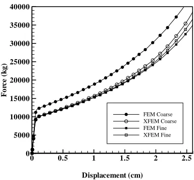
The component is modeled for the high reduction of 2.60 cm. In Figures 6 and 7, the deformed configurations are shown together with the normal stress σy distributions of compacted component at the final stage of die-pressing using both the X-FEM and FEM methods. In order to compare the results of two different techniques, the force-displacement curves are plotted in Figure 8 using X-FEM and FEM analyses. Remarkable agreements can be observed between two different methods. This example adequately presents the capability of X-FEM technique in 3D modeling of large elasto-plastic deformation of die-pressing problems.
(a)
[image:5.595.85.253.85.292.2](b)
Figure 7. The normal stress contours at the deformation of 2.60 cm
d= ; a) The X-FEM, b) The FEM
Displacement (cm)
Fo
rc
e
(k
g
)
0 0.5 1 1.5 2 2.5
0 5000 10000 15000 20000 25000 30000 35000 40000
FEM Coarse XFEM Coarse FEM Fine XFEM Fine
Figure 8. The variation of reaction force with displacement; A comparison between FEM and X-FEM analyses
C. Die Pressing of Shaped Tablet Component
The last example chosen demonstrates the performance of X-FEM technique in modeling large elasto-plastic deformation of shaped-tablet pressing, as shown in Figure 9. A shaped tablet is compacted by simultaneous action of top and bottom punches. This component is a challenging example for the proposed X-FEM approach because it involves two crossing interfaces; the first is the surface between punch and tablet and the second consists of the contact interface between the die and tablet. The punch and sleeve are both elastic and the tablet has a nonlinear elasto-plastic behavior. On the virtue of symmetry, the process is modeled for one-quarter of component.
In Figure 10, the X-FEM and FEM meshes are shown at the initial stage of compaction. In the X-FEM analysis, the discontinuity in different material properties of tablet and punch is modeled by level set function, and the discontinuity in contact interface between the die and tablet is simulated by the Heaviside enrichment function. In the FEM analysis, the finite element mesh is combined with the contact elements along the contact surface.
[image:5.595.63.279.506.714.2](a) (b)
[image:5.595.311.546.570.719.2](a) (b)
Figure 10. Die pressing of shaped tablet component; a) The X-FEM mesh, b) The FEM mesh
(a) (e)
[image:6.595.50.278.284.431.2](b) (f)
Figure 11. Die pressing of shaped tablet component; Deformed configuration at d=2.60 cm; a) The X-FEM, b) The FEM
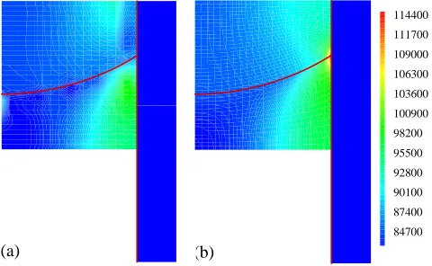
114400 111700 109000 106300 103600 100900 98200 95500 92800 90100 87400 84700
(e) (f)
Figure 12. The normal stress contours at the deformation of 2.60 cm
d= ; a) The X-FEM, b) The FEM
In Figure 11, the deformed X-FEM and FEM meshes are shown at the deformation of 2.60 cm. The distributions of the normal stress contour at the final stage of compaction are shown in Figure 12 for both techniques. Complete agreements can be observed between the X-FEM and FEM methods.
VII. CONCLUSION
In the present paper, the X-FEM method was presented in the framework of arbitrary Lagrangian-Eulerian formulation for large deformation of forming processes. The X-ALE-FEM technique was developed by implementation of the enrichment functions to approximate the displacement fields of elements located on discontinuity due to different material properties. The X-FEM method was applied by performing a splitting operator to separate the material (Lagrangian) phase from convective (Eulerian) phase. The Lagrangian phase was carried out by partitioning the domain with triangular sub-elements whose Gauss points were used for integration of the domain of the elements. The ALE governing equation was derived by substituting the relationship between the material time derivative and grid time derivative into the governing equations of continuum mechanics. The analysis was carried out according to Lagrangian phase at each time step until the required convergence is attained. The Eulerian phase was then applied to keep the mesh configuration regular.
The capability of proposed method was finally demonstrated through several numerical examples. The simulation of the deformation was shown as well as the distribution of stresses and the results were compared with those obtained by FEM analysis. Remarkable agreements were achieved between the X-FEM and FEM techniques. The results clearly indicate that the proposed approach can be efficiency used to model the large plastic deformation of forming problems.
REFERENCES
[1] A.R. Khoei, R.W. Lewis. Adaptive finite element remeshing in a large deformation analysis of metal powder forming, Int. J. Numer.
Meth. Engng., 1999; 45, pp. 801-820.
[2] A.R. Khoei, A.R. Azami, M. Anahid, R.W. Lewis. A three-invariant hardening plasticity for numerical simulation of powder forming processes via the arbitrary Lagrangian-Eulerian FE model. Int. J.
Numer. Meth. Engng., 2006; 66, pp. 843-877.
[3] A.R. Khoei, M. Anahid, K. Shahim. Arbitrary Lagrangian-Eulerian method in plasticity of pressure-sensitive material; Application to powder forming processes. Submitted to: Computational Mechanics, 2007.
[4] A.R. Khoei, A. Shamloo, A.R. Azami. Extended finite element method in plasticity forming of powder compaction with contact friction. Int. J. Solids Struct., 2006; 43, pp. 5421-5448.
[5] A.R. Khoei, M. Nikbakht. An enriched finite element algorithm for numerical computation of contact friction problems. Int. J. Mech.
Sciences, 2007; 49, pp. 183-199.
[6] A.R. Khoei, M. Anahid, K. Shahim. An extended arbitrary Lagrangian-Eulerian finite element method for large deformation of solid mechanics. Submitted to: Finite Elem. Anal. Design, 2007. [7] M. Anahid, A.R. Khoei. New development in extended finite element
modeling of large elasto-plastic deformations, Submitted to: Int. J. Numer. Meth. Engng., 2007.
[8] A.R. Khoei, S.O.R. Biabanaki, M. Anahid, Extended finite element method for three-dimensional large plasticity deformations. Submitted to: Comput. Meth. Appl. Mech. Eng., 2007.
[9] A.R. Khoei. Computational Plasticity in Powder Forming Processes,
Elsevier, UK, 2005.
[image:6.595.49.289.488.636.2]