Abstract—We introduce a new aggregation operator that unifies the weighted average and the ordered weighted averaging (OWA) operator in the same formulation. We call it the ordered weighted averaging – weighted averaging (OWAWA) operator. This aggregation operator provides a more complete representation of the weighted average and the OWA because it includes them as particular cases of a more general context. We study different properties and families of the OWAWA operator. We also develop an illustrative example of the new approach in a decision making problem about selection of strategies.
Index Terms—OWA operator; Weighted average; Decision making; Selection of strategies.
I. INTRODUCTION
The weighted average (WA) is one of the most common aggregation operators found in the literature. It can be used in a wide range of different problems including statistics, economics, engineering, etc. Another interesting aggregation operator that has not been used so much in the literature, especially because it appeared in 1988, is the ordered weighted averaging (OWA) operator [12]. The OWA operator provides a parameterized family of aggregation operators that range from the maximum to the minimum. For further reading on the OWA operator and some of its applications, refer to [1-4,6,8-19].
Recently, some authors [9-11] have tried to unify both concepts in the same formulation. It is worth noting the work developed by Torra [9] with the introduction of the weighted OWA (WOWA) operator and the work of Xu [11] about the hybrid averaging (HA) operator. Both models arrived to a unification between the OWA and the WA because both concepts were included in the formulation as particular cases. However, as it has been studied in [6], these models seem to be a partial unification but not a real one because they can unify them but they cannot consider how relevant these concepts are in the specific problem considered. For example, in some problems we may prefer to give more importance to the OWA operator because we believe that it is more relevant and vice versa.
In this paper, we present a new approach to unify the OWA operator with the WA. We call it the ordered weighted averaging – weighted averaging (OWAWA) operator. We could also refer to it as the WOWA operator but we have not
Manuscript received March 23, 2009.
J.M. Merigó is with the Department of Business Administration, University of Barcelona, Av. Diagonal 690, 08034 Barcelona, Spain (corresponding author: +34-93-4021962; fax: +34-93-4039882; e-mail: jmerigo@ ub.edu).
done so because in the literature there is another approach that already uses this name [9]. The main advantage of this approach is that it unifies the OWA and the WA taking into account the degree of importance of each case in the formulation. Thus, we are able to consider situations where we give more or less importance to the OWA and the WA depending on our interests and the problem analysed.
We study different properties of the OWAWA operator and different particular cases. We see that the OWA and the WA are particular cases of this general formulation. Moreover, we are also able to unify the arithmetic mean (or simple average) with the OWA operator when the weights of the WA are equal. We study other families such as the
step-OWAWA, the median-OWAWA, the
olympic-OWAWA, the S-OWAWA, the centered-OWAWA, etc.
We also analyze the applicability of the new approach and we see that it is possible to develop an astonishingly wide range of applications. The reason is that the OWAWA includes the WA and the OWA as special cases. Therefore, all the studies that use the WA or the OWA can be revised by using this new approach in order to obtain a more complete analysis of the problem analysed. For example, we can apply it in a lot of problems about statistics, economics, engineering, decision theory, etc. In this paper we focus on a decision making problem about selection of strategies. The main advantage of the OWAWA in these problems is that it is possible to consider the subjective probability (or the degree of importance) and the attitudinal character of the decision maker.
This paper is organized as follows. In Section 2 we briefly revise the WA and the OWA operator. In Section 3 we present the new approach. Section 4 analyzes different families of OWAWA operators. In Section 5 we study the applicability of the new approach in a decision making problem. Section 6 presents a numerical example and in Section 7 we summarize the main conclusions of the paper.
II. PRELIMINARIES
A. The OWA Operator
The OWA operator [12] is an aggregation operator that provides a parameterized family of aggregation operators between the minimum and the maximum. It can be defined as follows.
Definition 1. An OWA operator of dimension n is a mapping
OWA: Rn→ R that has an associated weighting vector W of dimension n such that wj∈ [0, 1] and ∑nj=1wj =1, then:
On the Use of the OWA Operator in the Weighted
Average and its Application in Decision Making
OWA(a1, …, an) = ∑
= n
j j j
b w
1
(1)
where bj is the jth largest of the ai.
Note that different properties can be studied such as the distinction between descending and ascending orders, different measures for characterizing the weighting vector and different families of OWA operators. Note that it is commutative, monotonic, bounded and idempotent. For further reading, refer, e.g., to [1-4,6,8-19].
B. The Weighted Average
The weighted average (WA) is one of the most common aggregation operators in the literature. It has been used in an incredible wide range of applications. It can be defined as follows.
Definition 2. A WA operator of dimension n is a mapping
WA: Rn→ R that has an associated weighting vector W, with
wj∈ [0, 1] and ∑nj=1wj = 1, such that
WA(a1, …, an) = ∑
= n
j j i
a w
1
(2)
where ai represents the argument variable.
The WA operator accomplishes the usual properties of the aggregation operators. For further reading on different extensions and generalizations of the WA, see for example [1-3,5-7,10-11].
III. THE ORDERED WEIGHTED AVERAGING - WEIGHTED AVERAGING OPERATOR
The ordered weighted averaging – weighted averaging (OWAWA) operator is a new model that unifies the OWA operator and the weighted average in the same formulation. Therefore, both concepts can be seen as a particular case of a more general one. This approach seems to be complete, at least as an initial real unification between OWA operators and WAs. It can also be seen as a unification between decision making problems under uncertainty (with OWA operators) and under risk (with probabilities).
Note that some previous models already considered the possibility of using OWA operators and WAs in the same formulation. The main models are the weighted OWA (WOWA) operator [9-10] and the hybrid averaging (HA) operator [11]. Although they seem to be a good approach, they are not so complete than the OWAWA because it can unify OWAs and WAs in the same model but they can not take in consideration the degree of importance of each case in the aggregation process. Moreover, in some particular cases we also find inconsistencies [6]. Other methods that could be considered are the concept of immediate probability [4,6,15,19]. This method is focused on the probability but it is easy to extend it to the use of WAs because sometimes the WA is used as a subjective probability. As said before, these an other approaches are useful for some particular situations but they does not seem to be so complete than the OWAWA because they can unify OWAs with WAs (or with probabilities) but they can not unify them giving different
degrees of importance to each case. Note that in future research we will also prove that these models can be seen as a special case of a general OWAWA operator (or its respective model with probabilities) that uses quasi-arithmetic means. Obviously, it is possible to develop more complex models of the WOWA, the HA and the IP-OWA that takes into account the degree of importance of the OWAs and the WAs (or probabilities) in the model but they seem to be artificial and not a natural unification as it will be shown below.
In the following, we are going to analyze the OWAWA operator. It can be defined as follows.
Definition 3. An OWAWA operator of dimension n is a
mapping OWAWA: Rn→ R that has an associated weighting vector W of dimension n such that wj ∈ [0, 1] and
∑n= =
j 1wj 1, according to the following formula:
OWAWA (a1, …, an) = ∑
= n
j j j
b v
1
ˆ (3)
where bj is the jth largest of the ai, each argument ai has an
associated weight (WA) vi with ∑ni=1vi = 1 and vi∈ [0, 1],
j j
j w v
vˆ =β +(1−β) with β ∈ [0, 1] and vj is the weight
(WA) vi ordered according to bj, that is, according to the jth
largest of the ai.
Note that it is also possible to formulate the OWAWA operator separating the part that strictly affects the OWA operator and the part that affects the WAs. This representation is useful to see both models in the same formulation but it does not seem to be as a unique equation that unifies both models.
Definition 4. An OWAWA operator is a mapping OWAWA: Rn → R of dimension n, if it has an associated weighting vector W, with ∑nj=1wj = 1 and wj∈ [0, 1] and a weighting
vector V that affects the WA, with ∑n=
i 1vi = 1 and vi∈ [0, 1],
such that:
OWAWA (a1, …, an) = ∑ + − ∑
= =
n
i i i n
j j j
a v b
w
1 1
) 1 ( β
β (4)
where bj is the jth largest of the arguments ai and β∈ [0, 1].
In the following, we are going to give a simple example of how to aggregate with the OWAWA operator. We consider the aggregation with both definitions.
Example 1. Assume the following arguments in an
13 . 0 1 . 0 7 . 0 2 . 0 3 . 0
ˆ1= × + × =
v 2 . 0 2 . 0 7 . 0 2 . 0 3 . 0
ˆ2 = × + × =
v 3 . 0 3 . 0 7 . 0 3 . 0 3 . 0
ˆ3= × + × =
v 37 . 0 4 . 0 7 . 0 3 . 0 3 . 0
ˆ4 = × + × =
v
And then, we calculate the aggregation process as follows: OWAWA = 0.13×60 + 0.2×50 + 0.3×30 + 0.37×20 = 34.2. With (4), we aggregate as follows:
OWAWA = 0.3 × (0.2 × 60 + 0.2 × 50 + 0.3 × 30 + 0.3 × 20) + 0.7 × (0.3 × 30 + 0.2 × 50 + 0.4 × 20 + 0.1 × 60) = 34.2. Obviously, we get the same results with both methods.
From a generalized perspective of the reordering step, it is possible to distinguish between the descending OWAWA (DOWAWA) and the ascending OWAWA (AOWAWA) operator by using wj = w*n−j+1, where wj is the jth weight of the
DOWAWA and w*n−j+1 the jth weight of the AOWAWA
operator.
If B is a vector corresponding to the ordered arguments bj,
we shall call this the ordered argument vector and WT is the transpose of the weighting vector, then, the OWAWA operator can be expressed as:
OWAWA (a1, …, an) = WTB (5)
Note that if the weighting vector is not normalized, i.e., W =∑n= ≠
j 1wj 1, then, the OWAWA operator can be expressed as:
OWAWA (a1, …, an) = ∑
= n
j j j
b v
W 1ˆ
1
(6)
The OWAWA is monotonic, commutative, bounded and idempotent. It is monotonic because if ai≥ ui, for all ai, then,
OWAWA(a1, a2,…, an) ≥ OWAWA(u1, u2…, un). It is
commutative because any permutation of the arguments has the same evaluation. That is, OWAWA(a1, a2,…, an) =
OWAWA(u1, u2,…, un), where (u1, u2,…, un) is any
permutation of the arguments (a1, a2,…, an). It is bounded
because the OWAWA aggregation is delimitated by the minimum and the maximum. That is, Min{ai} ≤ OWAWA(a1,
a2,…, an) ≤ Max{ai}. It is idempotent because if ai = a, for all
ai, then, OWAWA(a1, a2,…, an) = a.
Another interesting issue to analyze are the measures for characterizing the weighting vector W. Following a similar methodology as it has been developed for the OWA operator [6,12] we can formulate the attitudinal character, the entropy of dispersion, the divergence of W and the balance operator. Note that these measures affect the weighting vector W but not the WAs because they are given as some kind of objective information.
IV. FAMILIES OF OWAWA OPERATORS
First of all we are going to consider the two main cases of the OWAWA operator that are found by analyzing the coefficient
β. Basically, if β = 0, then, we get the WA and if β = 1, the
OWA operator. Note that if vi = 1/n, for all i, then, we get the
unification between the arithmetic mean (or simple average) and the OWA operator.
By choosing a different manifestation of the weighting vector in the OWAWA operator, we are able to obtain different types of aggregation operators. For example, we can obtain the partial maximum, the partial minimum, the partial average and the partial weighted average.
Remark 1. The partial maximum is found when w1 = 1 and wj
= 0 for all j ≠ 1. The partial minimum is formed when wn = 1
and wj = 0 for all j ≠ n. More generally, the step-OWAWA is
formed when wk = 1 and wj = 0 for all j ≠ k. Note that if k = 1,
the step-OWAWA is transformed to the partial maximum, and if k = n, the step-OWAWA becomes the partial minimum operator.
Remark 2. The partial average is obtained when wj = 1/n for
all j, and the partial weighted average is obtained when the ordered position of i is the same as the ordered position of j.
Remark 3. Another interesting family is the S-OWAWA
operator. It can be subdivided into three classes: the “or-like,” the “and-like” and the generalized S-OWAWA operators. The generalized S-OWAWA operator is obtained if w1 =
(1/n)(1 − (α + β)) + α, wn = (1/n)(1 − (α + β)) + β, and wj =
(1/n)(1 − (α + β)) for j = 2 to n − 1, where α, β∈ [0, 1] and α + β ≤ 1. Note that if α = 0, the generalized S-OWAWA operator becomes the “and-like” S-OWAWA operator, and if β = 0, it becomes the “or-like” S-OWAWA operator.
Remark 4. Another family of aggregation operator that could
be used is the centered-OWAWA operator. We can define an OWAWA operator as a centered aggregation operator if it is symmetric, strongly decaying and inclusive. Note that these properties have to be accomplished for the weighting vector
W of the OWAWA operator but not necessarily for the
weighting vector V of the WA. It is symmetric if wj = wj+n−1. It
is strongly decaying when i < j ≤ (n + 1)/2 then wi < wj and
when i > j ≥ (n + 1)/2 then wi < wj. It is inclusive if wj > 0. Note
that it is possible to consider a softening of the second condition by using wi≤ wj instead of wi < wj, and it is also
possible to remove the third condition. We shall refer to it as a non-inclusive centered-OWAWA operator.
Remark 5. For the median-OWAWA, if n is odd we assign w(n + 1)/2 = 1 and wj* = 0 for all others. If n is even we assign for
example, wn/2 = w(n/2) + 1 = 0.5 and wj* = 0 for all others. For the
weighted median-OWAWA, we select the argument bk that
has the kth largest argument such that the sum of the weights from 1 to k is equal or higher than 0.5 and the sum of the weights from 1 to k − 1 is less than 0.5.
Remark 6. Another type of aggregation that could be used is
the E-Z OWAWA weights. In this case, we should distinguish between two classes. In the first class, we assign wj* = (1/q)
for j* = 1 to q and wj* = 0 for j* > q, and in the second class,
we assign wj* = 0 for j* = 1 to n − q and wj* = (1/q) for j* = n
Remark 7. The olympic-OWAWA is generated when w1 = wn
= 0, and for all others wj* = 1/(n − 2). Note that it is possible to
develop a general form of the olympic-OWAWA by considering that wj = 0 for j = 1, 2, …, k, n, n − 1, …, n − k +
1, and for all others wj* = 1/(n − 2k), where k < n/2. Note that
if k = 1, then this general form becomes the usual olympic-OWAWA. If k = (n − 1)/2, then this general form becomes the median-OWAWA aggregation. That is, if n is odd, we assign w(n + 1) / 2 = 1, and wj* = 0 for all other values. If
n is even, we assign, for example, wn/2 = w(n / 2) + 1 = 0.5 and wj*
= 0 for all other values.
Remark 8. Note that it is also possible to develop the contrary
case, that is, the general olympic-OWAWA operator. In this case, wj = (1/2k) for j = 1, 2, …, k, n, n − 1, …, n − k + 1, and
wj = 0, for all other values, where k < n/2. Note that if k = 1,
then we obtain the contrary case for the median-OWAWA.
Remark 9. A further interesting type is the
non-monotonic-OWAWA operator. It is obtained when at least one of the weights wj is lower than 0 and ∑nj=1wj =1. Note that a key aspect of this operator is that it does not always achieve monotonicity. Therefore, strictly speaking, this particular case is not an OWAWA operator. However, we can see it as a particular family of operators that is not monotonic but nevertheless resembles an OWAWA operator.
Remark 10. Note that other families of OWAWA operators
could be used following the recent literature about different methods for obtaining the OWAWA weights such as [1-3,6,8,12,14,16].
V. SELECTION OF STRATEGIES WITH THE OWAWA OPERATOR
The OWAWA operator is applicable in a wide range of situations where it is possible to use the WA and the OWA operator. Therefore, we see that the applicability is incredibly broad because all the previous models, theories, etc., that uses the WA can be extended by using the OWAWA operator. The reason is that most of the problems with WAs deal with uncertainty. Usually, in most of the problems it is assumed a neutral attitudinal character against the WA but we are still under uncertainty. Thus, sometimes we may prefer to be more or less optimistic against this information. Moreover, by using the OWA in the WA, we can under or overestimate the results of a specific problem. Note also that the WA can be seen as a subjective probability.
Summarizing some of the main fields where it is possible to develop a lot of applications with the OWAWA operator, we can mention:
• Statistics. • Mathematics • Economics • Decision theory • Engineering • Physics • Etc.
Note that we can use the OWAWA operator in practically
all the previous studies that have used the WA or the OWA in the analysis. In this paper, we will consider a decision making application in the selection of strategies. The use of the OWAWA operator can be useful in a lot of situations, but the main reason for use it is when we want to consider the subjective probability (or degree of importance) of each state of nature (or characteristic) and the attitudinal character of the decision maker in the same problem.
The process to follow in the selection of strategies with the OWAWA operator is similar to the process developed in [5-6], with the difference that now we are considering a strategic management problem. The 5 steps of the decision process can be summarized as follows:
Step 1: Analysis and determination of the significant
characteristics of the available strategies for the company. Theoretically, it is represented as: C = {C1, C2,…, Ci,…, Cn},
where Ci is the ith characteristic of the strategy and we
suppose a limited number n of characteristics.
Step 2: Fixation of the ideal levels of each characteristic in
order to form the ideal strategy. Table 1: Ideal strategy
C1 C2 … Ci … Cn
P = µ1 µ2 … µi … µn
where P is the ideal strategy expressed by a fuzzy subset, Ci is
the ith characteristic to consider and µi ∈ [0, 1]; i = 1, 2, …, n,
is a number between 0 and 1 for the ith characteristic.
Step 3: Fixation of the real level of each characteristic for
all the strategies considered. Table 2: Available alternatives
C1 C2 … Ci … Cn
Pk = µ1(k) µ2(k) … µi(k) … µn(k)
with k = 1, 2, …, m; where Pk is the kth strategy expressed by
a fuzzy subset, Ci is the ith characteristic to consider and µi(k)
∈ [0, 1]; i = 1, …, n, is a number between 0 and 1 for the ith characteristic of the kth strategy.
Step 4: Comparison between the ideal strategy and the
different alternatives considered using the OWAWA operator. In this step, the objective is to express numerically the removal between the ideal strategy and the different alternatives considered. Note that it is possible to consider a wide range of OWAWA operators such as those described in Section 3 and 4.
Step 5: Adoption of decisions according to the results
found in the previous steps. Finally, we should take the decision about which strategy select. Obviously, our decision is to select the strategy with the best results according to the type of OWAWA operator used in the analysis.
VI. NUMERICAL EXAMPLE
• A1 = Develop a strong expansive monetary policy.
• A2 = Develop an expansive monetary policy.
• A3 = Do not develop any change in the monetary
policy.
• A4 = Develop a contractive monetary policy.
• A5 = Develop a strong contractive monetary policy.
In order to evaluate these strategies, the government has brought together a group of experts. This group considers that the key factor is the economic situation of the world economy for the next period. They consider 5 possible states of nature that could happen in the future:
• S1 = Very bad economic situation.
• S2 = Bad economic situation.
• S3 = Regular economic situation.
• S4 = Good economic situation.
• S5 = Very good economic situation.
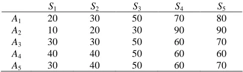
The results of the available strategies, depending on the state of nature Si and the alternative Ak that the decision maker
[image:5.595.304.547.214.290.2]chooses, are shown in Table 1. Table 1: Available alternatives
S1 S2 S3 S4 S5
A1 20 30 50 70 80
A2 10 20 30 90 90
A3 30 30 50 60 70
A4 40 40 50 60 60
A5 30 40 50 60 70
In this problem, the experts assume the following weighting vector: W = (0.3, 0.2, 0.2, 0.2, 0.1). They assume that the WA that each state of nature will have is: V = (0.1, 0.2, 0.3, 0.3, 0.1). Note that the OWA operator has an importance of 40% and the probabilistic information an importance of 60%. For doing so, we will use Eq. (3) to calculate the OWAWA aggregation. The results are shown in Table 2. Table 2: OWAWA weights
1 ˆ
v vˆ2 vˆ3 vˆ4 vˆ5
V* 0.18 0.2 0.26 0.26 0.1
With this information, we can aggregate the expected results for each state of nature in order to make a decision. In Table 3, we present different results obtained by using different types of OWAWA operators.
Table 3: Aggregated results
WA OWA WAM OWAWA
A1 52 56 52.4 53.6
A2 50 57 51.6 52.8
A3 49 52 49.6 50.2
A4 51 52 50.8 51.4
A5 51 54 51.6 52.2
Note that we can also obtain these results by using Eq. (4). Then, we will calculate separately the OWA and the probabilistic approach as shown in Table 4.
Table 4: First aggregation process
WA AM OWA
A1 52 50 56
A2 50 48 57
A3 49 48 52
A4 51 50 52
A5 51 50 54
After that, we will aggregate both models in the same process considering that the OWA model has a degree of importance of 40% and the probabilistic information 60% as shown in Table 5.
Table 5: Final aggregated results
WA OWA WAM OWAWA
A1 52 56 52.4 53.6
A2 50 57 51.6 52.8
A3 49 52 49.6 50.2
A4 51 52 50.8 51.4
A5 51 54 51.6 52.2
Obviously, we get the same results with both methods. If we establish an ordering of the alternatives, a typical situation if we want to consider more than one alternative, then, we get the results shown in Table 6. Note that the first alternative in each ordering is the optimal choice.
Table 6: Ordering of the strategies
Ordering WA A1A4=A5A2A3
OWA A2A1A5A3=A4
WAM A1A2=A5A4A3
OWAWA A1A2A5A4A3
As we can see, depending on the aggregation operator used, the ordering of the strategies may be different. Therefore, the decision about which strategy select may be also different.
VII. CONCLUSION
We have developed a new aggregation operator that unifies the WA with the OWA operator. We have called it the OWAWA operator. The main advantage is that it provides a unified framework between the WA and the OWA that allows us to use both of them in the same formulation and considering how relevant they are in the specific problem considered. We have studied some of its main properties and we have seen that it is possible to use a wide range of particular cases in the OWAWA operator.
[image:5.595.47.289.351.423.2]the OWAWA operator because we are able to consider WAs and OWAs at the same time.
In future research, we expect to develop further extensions to this approach by adding new characteristics in the problem such as the use of order inducing variables, uncertain information (interval numbers, fuzzy numbers, linguistic variables, etc.), generalized and quasi-arithmetic means and distance measures. We will also extend this approach to situations where we use the probability instead of the WA and further developments that have been initially developed in [6]. We will also consider different applications giving special attention to business decision making problems such as investment and product management.
REFERENCES
[1] G. Beliakov, A. Pradera and T. Calvo, Aggregation Functions: A
Guide for Practitioners. Berlin: Springer-Verlag, 2007.
[2] H. Bustince, F. Herrera and J. Montero, Fuzzy Sets and Their
Extensions: Representation, Aggregation and Models. Berlin:
Springer-Verlag, 2008.
[3] T. Calvo, G. Mayor and R. Mesiar, Aggregation Operators: New
Trends and Applications. New York: Physica-Verlag, 2002.
[4] K.J. Engemann, D.P. Filev and R.R. Yager, Modelling decision making using immediate probabilities. International Journal of General Systems, 24:281-294, 1996.
[5] J. Gil-Aluja, The interactive management of human resources in
uncertainty. Dordrecht: Kluwer Academic Publishers, 1998.
[6] J.M. Merigó, New extensions to the OWA operators and its
application in decision making (In Spanish). PhD Thesis, Department
of Business Administration, University of Barcelona, 2008.
[7] J.M. Merigó and A.M. Gil-Lafuente, Unification point in methods for the selection of financial products. Fuzzy Economic Review, 12:35-50, 2007.
[8] J.M. Merigó and A.M. Gil-Lafuente, The induced generalized OWA operator. Information Sciences, 179:729-741, 2009.
[9] V. Torra, The weighted OWA operator. International Journal of
Intelligent Systems, 12:153-166, 1997.
[10] V. Torra and Y. Narukawa, Modeling Decisions: Information Fusion
and Aggregation Operators. Berlin: Springer-Verlag, 2007.
[11] Z.S. Xu and Q.L. Da, An overview of operators for aggregating information. International Journal of Intelligent Systems, 18:953-968, 2003
[12] R.R. Yager, On ordered weighted averaging aggregation operators in multi-criteria decision making. IEEE Transactions on Systems, Man
and Cybernetics B, 18:183-190, 1988.
[13] R.R. Yager, Decision making under Dempster-Shafer uncertainties.
International Journal of General Systems, 20:233-245, 1992.
[14] R.R. Yager, Families of OWA operators. Fuzzy Sets and Systems, 59:125-148, 1993.
[15] R.R. Yager, Including decision attitude in probabilistic decision making. International Journal of Approximate Reasoning, 21:1-21, 1999.
[16] R.R. Yager, Centered OWA operators, Soft Computing, 11:631-639, 2007.
[17] R.R. Yager and D.P. Filev, Parameterized “andlike” and “orlike” OWA operators. International Journal of General Systems, 22:297-316, 1994.
[18] R.R. Yager and D.P. Filev, Induced ordered weighted averaging operators. IEEE Transactions on Systems, Man and Cybernetics B, 29:141-150, 1999.
[19] R.R. Yager and J. Kacprzyk, The Ordered Weighted Averaging
Operators: Theory and Applications. Norwell: Kluwer Academic